


1. Introduction
Difficulties in the locomotion of humanoid robots include how to represent the dynamics of the robot [Reference Yamamoto, Kamioka and Sugihara39] and how to control the inherently unstable dynamics [Reference Al-Shuka, Corves, Zhu and Vanderborght1, Reference Moro and Sentis24, Reference Sugihara and Morisawa34]. Recent strategies have integrated whole-body dynamics models into both the planner [Reference Lee, Bakolas and Sentis22, Reference Posa, Cantu and Tedrake27] and the controller [Reference Koolen, Bertrand, Thomas, de Boer, Wu, Smith, Englsberger and Pratt20, Reference Romualdi, Dafarra, Hu, Ramadoss, Chavez, Traversaro and Pucci30], addressing these issueseffectively.However, while these methods enhance stability and accommodate a variety of motions, they require extensive computational resources, making online planning for extended durations difficult. In contrast, reduced-order models present a more traditional yet robust approach, enabling effective planning and control with greater simplicity and reduced computational cost.
Original control methods using reduced-order models such as the linear inverted pendulum (LIP) [Reference Kajita, Kanehiro, Kaneko, Fujiwara, Harada, Yokoi and Hirukawa13], spring-loaded inverted pendulum (SLIP) [Reference Raibert29], and inverted pendulum (IP) models [Reference Hodgins10, Reference Li and Chen23] govern robot locomotion through intermittent control inputs. Motion during longer locomotion phases (e.g., the single support (SS) phase of walking or the flight phase of running) is governed by zero inputs to the model (no control), while motion during other short phases is controlled through feedback inputs, such as foot placement and kicking. In other words, these controllers intermittently apply control inputs and can thus be referred to as ”intermittent controllers” [Reference Craik4, Reference Fu, Suzuki, Kiyono, Morasso and Nomura8]. During the longer phase, models like LIP generate specific forces (model’s force) that yield closed-form solutions to the equations of motion (EoM). Consequently, the motion in the longer phase is uniquely determined, while feedback inputs during the short phase facilitate precise control of the robot’s motion. Here, this phase has no control input except the model’s force, then, we refer to this as zero input and/or no control. These intermittent control strategies, leveraging models with closed-form solutions, are powerful tools due to their low computational complexity. Moreover, these controllers allow robots to follow the natural dynamics of the model itself, enabling energetically and computationally efficient walking.
For example, the original LIP model control method using ”orbital energy” [Reference Kajita, Yamaura and Kobayashi14], the extended LIP model control method using ”capture point” [Reference Pratt, Carff, Drakunov and Goswami28], and the SLIP model control method (widely known as the Raibert controller) [Reference Hodgins10, Reference Raibert29] are all examples of intermittent controllers. Kajita et al. proposed the concept of orbital energy, a conserved energy form that modulates energy at switching times, and the positions of foot touchdowns to control walking speed [Reference Kajita, Yamaura and Kobayashi14]. Similarly, Pratt et al. introduced the capture point, the location, and the timing of foot placement required to stop the robot in an upright posture. This point is derived by solving for when the orbital energy equals zero and is used to adjust foot touchdown positions to control walking speed [Reference Pratt, Carff, Drakunov and Goswami28]. Both approaches employ intermittent feedback controllers to adjust leg touchdown positions. Additionally, the Raibert controller for running incorporates kick control just before the foot leaves the ground into a feedback controller, along with foot placement control [Reference Raibert29, Reference Sayyad, Seth and Seshu32]. While similar to other controllers in some ways, this method is simple and versatile, extending to various robotic gait motions, including both running and walking [Reference Hodgins10].
These intermittent controllers for walking are supposed to follow models such as LIP, IP, or SLIP. Therefore, during the longer phase, the robot is required to generate the specified force to follow the model without any other additional forces. However, humanoid robots generate angular momentum through upper body and limb movements, especially during swing motions, generating additional force. In practical implementation, to ignore the momentum, robots often use very lightweight legs to align with these models [Reference Hubicki, Grimes, Jones, Renjewski, Spröwitz, Abate and Hurst11, Reference Kajita, Yamaura and Kobayashi14, Reference Raibert29, Reference Xiong and Ames38]. Robot hardware designed to minimize discrepancies in the walking model ensures that the controller does not need to correct model errors. However, developing these ultralight legs for full-sized humanoid robots is very difficult. Even when the leg mass is significantly less than the total body mass (e.g., total body mass to swing-leg mass ratio = 10:1 [Reference Kamioka, Shin, Yamaguchi and Muromachi15]), the angular momentum arising from its swing motion cannot be ignored.
A recent trend in control frameworks involves methods that include a center of mass (CoM) controller and a whole-body stabilizer [Reference Sugihara and Morisawa34]. In such frameworks, both the controller and the stabilizer continuously calculate control inputs (referred to as the ”continuous feedback controller”), while the whole-body stabilizer compensates for inaccuracies caused by modeling errors in reduced-order models. However, this continuous feedback control approach often leads to energetically inefficient movements due to additional compensatory actions, resulting in higher energy consumption and significant computational cost. Furthermore, recent studies have shifted toward sequentially optimizing centroidal dynamics that consider angular momentum [Reference He, Wu, Zhang, Zhang, Shi, Liu, Sun, Su and Leng9, Reference Orin, Goswami and Lee25]. While these methods enable the generation of diverse trajectories by accounting for the angular momentum of the robot’s limbs and upper body, they make it difficult to obtain closed-form solutions of the EoM, thereby increasing the computational resources required for trajectory planning. Although the intermittent controller offers reduced energy consumption and computational cost by applying control inputs only at discrete intervals, it has not been widely adopted recently. One major challenge is that the intermittent controller is more affected by modeling errors compared to the latest approaches. During its no-control duration, stability heavily relies on the accuracy of the model. Most models used for intermittent control assume zero angular momentum; however, actual humanoid robots generate angular momentum through upper body and limb movements, especially during rapid swing motions.
To address these issues, some studies have proposed multi-mass models by adding additional masses to the base model (e.g., the LIP model [Reference Ding, Zhou, Guo and Xiao5, Reference Kasaei, Ahmadi, Lau and Pereira16, Reference Kasaei, Ahmadi, Lau and Pereira17, Reference Takenaka, Matsumoto and Yoshiike36] or the SLIP model [Reference Pelit, Chang, Takano and Yamakita26]). However, the coupled dynamics between the base model’s CoM and the additional masses render the models nonlinear, necessitating the determination of the trajectories for each additional mass before calculating the CoM trajectory [Reference Eslami, Yousefi-Koma and Khadiv6, Reference Sato, Sakaino and Ohnishi31, Reference Shimmyo, Sato and Ohnishi33, Reference Takenaka, Matsumoto and Yoshiike36]. Although these computations are feasible with numerical integration of the EoM, they require iterative calculations to attain the target behavior, and variations in the integration paths can lead to incremental errors in the model. Most models rely on closed-form solutions derived from single-mass models [Reference Kasaei, Ahmadi, Lau and Pereira17] or adopt multi-mass representations without such solutions [Reference Pelit, Chang, Takano and Yamakita26], requiring compensatory controllers to address modeling inaccuracies and complicating the design of intermittent control strategies. In other cases, imposing a constant height condition on both the base model and additional masses can linearize the dynamics, enabling closed-form solutions. However, this approach forces a constant height for the swing-leg CoM, resulting in an unrealistic shuffle gait for the robot [Reference Faraji and Ijspeert7]. Consequently, these methods often produce unrealistic trajectories or cannot provide closed-form solutions for the EoM. To apply the intermittent controller, it is essential to have a model for which the EoM can be analytically solved, even for the motion of a multi-mass model. If constraints could be devised that allow the model’s EoM, incorporating angular momentum generated by leg inertia, to have closed-form solutions, it would eliminate the need to unrealistically reduce leg mass and implement inefficient corrections, potentially enabling robot behavior to be controlled through a straightforward intermittent controller.
In this paper, we propose a multi-mass model with a closed-form solution, consisting of an IP mass and an additional mass for the swing leg, and an intermittent control method for this model, as illustrated in Figure 1(c). We focus on the fact that a conservative system has a closed-form solution for the EoM, providing the conditions under which the multi-mass system becomes a conservative system by imposing holonomic constraints on the trajectories of the additional masses (specifically the swing-leg CoM) during the SS phase. This modeling during the SS phase allows the robot to uniquely define its behavior without feedback control, and the feedback controller during the double support (DS) phase preceding the SS phase enables it to control walking behavior during the SS phase. In the numerical simulation, we analyze the system energy during walking to verify that the model forms a conservative system, resulting in the energy value becoming constant. Furthermore, we demonstrate simulations and robot experiments to evaluate the intermittent controller. The results show that our intermittent controller allows tracking the target walking speed, although previous intermittent control methods have difficulty tracking it.

Figure 1. Definition of mass model and the proposed constrained model. Panel (a) displays a multi-mass model. Panel (b) indicates an overview of the constrained position trajectory in the proposed method. Parameter definitions are shown in Table I.
The main contributions of this work are as follows:
-
1. Multi-mass model with closed-form solution: We introduce a dynamical system with a closed-form solution of the EoM by forming a conservative system (Section 2.2) and propose a model that allows for the adjustment of swing leg trajectories (Section 3.2).
-
2. Intermittent walking controller: We develop an intermittent walking controller based on the multi-mass model, enabling walking behavior control through zero input during the SS phase and feedback control during the DS phase (Section 3.3).
-
3. Walking velocity trackability: Our controller maintains a conservative system during the SS phase, preserving constant energy, and tracks the target walking velocity (Sections 4.1.1, 4.1.2, and 4.2).
-
4. Trajectory variety and stability: Our controller supports a variety of swing leg trajectories (Section 4.1.2 and Appendix G) and demonstrates stability by returning to the target walking velocity under external disturbances (Section 4.2).
2. Preliminary
This section introduces related studies and fundamental dynamics necessary for the intermittent controller of bipedal robots. First, existing models that feature closed-form solutions of the EoM are introduced. Next, the dynamic properties required to extend this method to general robots with a multi-mass model are described.
2.1. Reduced-order models with closed-form solutions for the equations of motion
Typical reduced-order models used in walking planners, such as the IP and LIP models, feature closed-form solutions for their EoMs [Reference Kajita, Hirukawa, Harada and Yokoi12]. The SLIP model, depicted in Figure 2(a), primarily applied to running, also admits a closed-form solution for the EoM during the flight phase, although obtaining a closed-form solution for the stance phase remains challenging. These models rely on forces generated by holonomic constraints between the CoM and the foot contact point. Under specific conditions, these holonomic constraint forces enable closed-form solutions.

Figure 2. Typical reduced-order models. panel (a) shows examples of reduced-order models that abstract bipedal locomotion. panel (b) shows the definition of mass model.
Typical models, such as the LIP model [Reference Kajita, Yamaura and Kobayashi14] and the IP model [Reference Kajita, Hirukawa, Harada and Yokoi12], exhibit linear trajectories in their respective coordinate systems (LIP: Cartesian coordinates, IP: polar coordinates). As a result, the EoMs of these models are expressed as second-order linear differential equations, as shown below:
 \begin{align} LIP &:\;\;\ddot {x} = \frac {g}{h} x,\;\;\;\;\;\;\;\; f = m g / \cos {\theta }, \end{align}
 \begin{align} IP &:\;\; \ddot {\theta } = \frac {g}{l_0} \sin {\theta },\;\;\; f = m g \cos {\theta } - m l_0 \dot {\theta }^2, \end{align}
where
 $g$
and
$g$
and
 $m$
denote gravitational acceleration and mass, respectively;
$m$
denote gravitational acceleration and mass, respectively;
 $x$
and
$x$
and
 $h$
represent the CoM position and height in the LIP model;
$h$
represent the CoM position and height in the LIP model;
 $l_0$
denotes the pendulum length in the IP model; and
$l_0$
denotes the pendulum length in the IP model; and
 $\theta$
and
$\theta$
and
 $f$
represent the pendulum angle and the force applied to the CoM. These variables are illustrated in Figure 2(a). Notably, the EoM of the SLIP model during the flight phase is also represented by a second-order linear differential equation with a constant gravitational force. Consequently, the EoMs of these models admit closed-form solutions.
$f$
represent the pendulum angle and the force applied to the CoM. These variables are illustrated in Figure 2(a). Notably, the EoM of the SLIP model during the flight phase is also represented by a second-order linear differential equation with a constant gravitational force. Consequently, the EoMs of these models admit closed-form solutions.
The CoM trajectory derived from models with closed-form solutions simplifies the estimation of future states. In scenarios without additional forces other than
 $f$
, as shown in Figure 2(a), the model’s trajectory can be uniquely determined by the closed-form solution, independent of the integration path. These models have enabled the development of various controllers that facilitate trajectory planning and stabilization. Notable examples include controllers based on orbital energy [Reference Kajita, Yamaura and Kobayashi14] and divergent components of motion [Reference Takenaka, Matsumoto and Yoshiike36].
$f$
, as shown in Figure 2(a), the model’s trajectory can be uniquely determined by the closed-form solution, independent of the integration path. These models have enabled the development of various controllers that facilitate trajectory planning and stabilization. Notable examples include controllers based on orbital energy [Reference Kajita, Yamaura and Kobayashi14] and divergent components of motion [Reference Takenaka, Matsumoto and Yoshiike36].
2.2. Alternative derivation for reduced-order model to yield closed-form solution
To construct a model that allows for closed-form solutions of the EoM, shaping the differential equations into a specific form is often required, typically using an intuitive approach [Reference Kajita, Yamaura and Kobayashi14, Reference Tazaki37]. Therefore, the trajectory of the model was significantly constrained, which made it difficult to design arbitrary trajectories and multi-mass models. On the other hand, focusing on the energy transformations described by the EoM, forming a conservative system (equivalent to having ”constant of motion” and ”conserved energy”) is a sufficient condition for a model to yield a closed-form solution of the EoM. Both the LIP model (1a) and the IP model (1b), which yield closed-form solutions of the EoM, are conservative systems. Therefore, as an alternative approach to obtaining models with closed-form solutions, the concept of the conservative system is essential, and modeling the targeted dynamics as a conservative system is key for constructing the intermittent control method. The following section introduces the EoM of a single-mass model, explains how to construct a conservative system for the EoM, and provides detailed examples of models with a conservative system.
First, we introduce the EoM of a single-mass model, with its mass and position denoted as
 $m_p$
and
$m_p$
and
 $\boldsymbol{p}{_p}$
, respectively. The EoM for this model, with an external force
$\boldsymbol{p}{_p}$
, respectively. The EoM for this model, with an external force
 $\boldsymbol{f}$
and moment
$\boldsymbol{f}$
and moment
 $\boldsymbol{\tau}$
applied to the CoM position, are as follows:
$\boldsymbol{\tau}$
applied to the CoM position, are as follows:
 \begin{align} m_{p}\ddot{\boldsymbol{p}}_{p} &= m_{p} \boldsymbol{g} + \boldsymbol{f}, \end{align}
 \begin{align} I_{p} \ddot {\boldsymbol \theta }_{p} &= \boldsymbol{\tau}, \end{align}
where
 $m_p$
,
$m_p$
,
 $I_p$
, and
$I_p$
, and
 $\boldsymbol{g}$
represent the mass, inertia, and gravitational acceleration for the CoM, respectively, as shown Figure 2(b).
$\boldsymbol{g}$
represent the mass, inertia, and gravitational acceleration for the CoM, respectively, as shown Figure 2(b).
 $\dot {\boldsymbol \theta }_{p}$
represents the angular velocity around the CoM. Assuming that the external force
$\dot {\boldsymbol \theta }_{p}$
represents the angular velocity around the CoM. Assuming that the external force
 $\boldsymbol{f}$
and moment
$\boldsymbol{f}$
and moment
 $\boldsymbol{\tau}$
generated within the system can be designed arbitrarily, (2a) and (2b) can describe the centroidal dynamics for any single-mass model [Reference Kajita, Hirukawa, Harada and Yokoi12].
$\boldsymbol{\tau}$
generated within the system can be designed arbitrarily, (2a) and (2b) can describe the centroidal dynamics for any single-mass model [Reference Kajita, Hirukawa, Harada and Yokoi12].
Second, we present how to form a conservative system for the EoM. By multiplying (2a) by
 $\dot {\boldsymbol{p}}_{p}$
and (2b) by
$\dot {\boldsymbol{p}}_{p}$
and (2b) by
 $\dot {\boldsymbol{\theta }}_{p}$
, their time-integral quantities represent energy. The total system energy can then be calculated as follows:
$\dot {\boldsymbol{\theta }}_{p}$
, their time-integral quantities represent energy. The total system energy can then be calculated as follows:
 \begin{align} E_{\textrm { mec}} = \frac {1}{2} m_{p} \dot {\boldsymbol{p}}_{p}^T\dot {\boldsymbol{p}}_{p} + \frac {1}{2} I_{p} \dot {\boldsymbol \theta }_{p}^T\dot {\boldsymbol \theta }_{p} + m_{p} \boldsymbol{g}^T \boldsymbol{p}_{p} - \int \boldsymbol{f}^T \dot {\boldsymbol{p}}_{p} dt - \int \boldsymbol{\tau}^T \dot {\boldsymbol \theta }_{p} dt. \end{align}
When the closed-form solution for energy is a time-independent function, the quantity
 $E_{\textrm { mec}}$
becomes a conserved quantity (conserved energy) with a constant value. In the case of unknown
$E_{\textrm { mec}}$
becomes a conserved quantity (conserved energy) with a constant value. In the case of unknown
 $\boldsymbol{f}$
and
$\boldsymbol{f}$
and
 $\boldsymbol{\tau}$
,
$\boldsymbol{\tau}$
,
 $E_{\textrm { mec}}$
, as shown in (3), includes a time-dependent term. If this term can be resolved in a time-independent manner, the energy in (3) becomes constant, representing a constant of motion and conserved energy. Thus, even for a model where the system itself generates external forces, the dynamical system of the model is considered conservative if both
$E_{\textrm { mec}}$
, as shown in (3), includes a time-dependent term. If this term can be resolved in a time-independent manner, the energy in (3) becomes constant, representing a constant of motion and conserved energy. Thus, even for a model where the system itself generates external forces, the dynamical system of the model is considered conservative if both
 $\int \boldsymbol{f}^T \dot {\boldsymbol{p}}_{p}dt$
and
$\int \boldsymbol{f}^T \dot {\boldsymbol{p}}_{p}dt$
and
 $\int \boldsymbol{\tau}^T \dot {\boldsymbol{\theta }}_{p}dt$
are independent of time.
$\int \boldsymbol{\tau}^T \dot {\boldsymbol{\theta }}_{p}dt$
are independent of time.
Last, we introduce example models with dynamical systems that form conservative systems. Given specific forms of conditions (the left-hand side of the equation), the energy of the external force and moment can be represented as time-independent terms:
 \begin{align} &\boldsymbol{f} = {j}(\boldsymbol{p}_{p}) \; \land \; {J}(\boldsymbol{p}_{p}) = \int {j}(\boldsymbol{p}_{p}) d \boldsymbol{p}_{p} \quad \Rightarrow \quad \int {f}^T \dot {\boldsymbol{p}}_{p} dt = J(\boldsymbol{p}_{p}) +Const, \end{align}
 \begin{align} &\boldsymbol{\tau} = {q}(\boldsymbol{\theta }_{p}) \; \land \; {Q}(\boldsymbol{\theta }_{p}) = \int {q}(\boldsymbol{\theta }_{p}) d \boldsymbol{\theta }_{p} \;\;\quad \Rightarrow \quad \int \boldsymbol{\tau}^T \dot {\boldsymbol \theta }_{p} dt = Q(\boldsymbol{\theta }_{p}) +Const. \end{align}
Examples such as the LIP and IP models, which incorporate the constraint forces (1a) and (1b) providing holonomic constraints, result in conservative systems, as illustrated in the following examples:
 \begin{align} \text {LIP:} \quad &E_{\text {mec}} = \frac {1}{2}m\dot {x}^2 - \frac {1}{2}m\frac {g}{h}x^2 = \text {Const} \quad \quad \; \Rightarrow \quad x = \pm \sqrt {\frac {h}{g}\dot {x}^2 - \frac {2h}{mg}E_{\text {mec}}}, \end{align}
 \begin{align} \text {IP:} \quad &E_{\text {mec}} = \frac {1}{2}ml_0^2\dot {\theta }^2 - mgl_0\cos \theta = \text {Const} \quad \Rightarrow \quad \theta = \arccos \left (\frac {l_0}{2g}\dot {\theta }^2 - \frac {E_{\text {mec}}}{mgl_0} \right ), \end{align}
where
 $l_0$
is the support leg length of the IP model. Note that these equations represent the conserved energy and the solution of the EoM; however, the primary significance lies in forming a conservative system, which ensures that the solution to the EoM is uniquely determined, rather than focusing solely on solving the EoM explicitly. Applying appropriate holonomic constraints allows the development of a model with a closed-form solution of the EoM for a multi-mass model, enabling intermittent control, including motions that generate additional external forces, such as swing motions.
$l_0$
is the support leg length of the IP model. Note that these equations represent the conserved energy and the solution of the EoM; however, the primary significance lies in forming a conservative system, which ensures that the solution to the EoM is uniquely determined, rather than focusing solely on solving the EoM explicitly. Applying appropriate holonomic constraints allows the development of a model with a closed-form solution of the EoM for a multi-mass model, enabling intermittent control, including motions that generate additional external forces, such as swing motions.
3. Proposed method
This section describes our proposed method, which includes modeling approaches for the intermittent controller aimed at making the motion during the SS phase a conservative system by applying holonomic constraints to a multi-mass model, including swing-leg motion. An overview is shown in Figure 3. First, we present the EoM and energy equation for a pendulum mass model with an additional mass. Next, we explain the conditions under which the dynamical system of the model becomes a conservative system. Lastly, we outline the implementation of a swing trajectory during the SS phase and the control strategy for regulating the robot’s walking speed by adjusting the kicking energy during the DS phase.

Figure 3. Overview of robot control. The ”robot” corresponds to Section 3.1 in numerical simulations and to the actual robot in experiments. The ”planner model,” which includes the swing-leg trajectory described in Section 3.2, is implemented as described in Section 3.3.1. The ”kick controller” is detailed in Section 3.3.2. In this paper, ”zero input” refers to the absence of control input applied to the model.
3.1. Equation of motion and energy for multi-mass model
A multi-mass model consists of a base single mass and an additional mass, as shown in Figure 1(b), with variables listed in Table I. The positions of these masses are denoted as
 $\boldsymbol{p}_{p}$
and
$\boldsymbol{p}_{p}$
and
 $\boldsymbol{p}_{a}$
, respectively. The pendulum mass represents the partial CoM of the robot, excluding the swing leg. In addition,
$\boldsymbol{p}_{a}$
, respectively. The pendulum mass represents the partial CoM of the robot, excluding the swing leg. In addition,
 $\boldsymbol{\theta }_{p}$
denotes the angular component of the single mass in the polar coordinate system. Under the assumption:
$\boldsymbol{\theta }_{p}$
denotes the angular component of the single mass in the polar coordinate system. Under the assumption:
Assumption 1. The foot is in contact with the ground during the SS phase,
the angular component
 $\boldsymbol{\theta }_{p}$
represents the support leg angle, as shown in Figure 1(b). Hereinafter, we define the mass of the single mass as the ”pendulum mass.” It should also be noted that more than two additional masses can be added. Let the force and moment required to represent the pendulum mass model be
$\boldsymbol{\theta }_{p}$
represents the support leg angle, as shown in Figure 1(b). Hereinafter, we define the mass of the single mass as the ”pendulum mass.” It should also be noted that more than two additional masses can be added. Let the force and moment required to represent the pendulum mass model be
 $\boldsymbol{f}_{s}$
and
$\boldsymbol{f}_{s}$
and
 $\boldsymbol{\tau}_s$
and let the force and moment from the additional mass to the pendulum mass be
$\boldsymbol{\tau}_s$
and let the force and moment from the additional mass to the pendulum mass be
 $\boldsymbol{f}_{r}$
and
$\boldsymbol{f}_{r}$
and
 $\boldsymbol{\tau}_{r}$
, respectively. The forces and moments acting on the pendulum mass are as follows:
$\boldsymbol{\tau}_{r}$
, respectively. The forces and moments acting on the pendulum mass are as follows:
 \begin{align} \boldsymbol{f} &= \boldsymbol{f}_{r} + \boldsymbol{f}_{s}, \end{align}
 \begin{align} \boldsymbol{\tau} &=\boldsymbol{\tau}_{r} + \tau _s . \end{align}
Note that in the case of point contact, moments generated at the CoM are essentially converted into translational forces, resulting in
 $\tau _s = 0$
. Furthermore, in most cases, the CoM-ZMP model is employed as the support leg model [Reference Sugihara, Yamane, Goswami and Vadakkepat35], meaning no moments arise from the representative ground contact point. Additionally, as our robot uses a point-contact leg design, the following assumption is introduced:
$\tau _s = 0$
. Furthermore, in most cases, the CoM-ZMP model is employed as the support leg model [Reference Sugihara, Yamane, Goswami and Vadakkepat35], meaning no moments arise from the representative ground contact point. Additionally, as our robot uses a point-contact leg design, the following assumption is introduced:
Assumption 2. No moments are generated from the assumed contact point.
A similar assumption holds for systems without point contact if the ZMP is considered the contact point of the support leg. Furthermore, the dynamics model of the pendulum mass (
 $f_s$
) corresponds to models such as (1a) or (1b). In this study, the IP model is adopted.
$f_s$
) corresponds to models such as (1a) or (1b). In this study, the IP model is adopted.
Table I. List of variables and parameters. Each position is a two-dimensional vector as
 $\boldsymbol{p}_*=[x_*, y_*]$
.
$\boldsymbol{p}_*=[x_*, y_*]$
.
Then, the EoM of the multi-mass model is derived by substituting (6a) and (6b) into (2a) and (2b), respectively. The resulting force
 $\boldsymbol{f}_{r}$
and moment
$\boldsymbol{f}_{r}$
and moment
 $\boldsymbol{\tau}_{r}$
are expressed as follows:
$\boldsymbol{\tau}_{r}$
are expressed as follows:
 \begin{align} \boldsymbol{f}_{r} &= -m_{a} \left (\ddot {\boldsymbol{p}}_{a} + \boldsymbol{g} \right ), \end{align}
 \begin{align} \boldsymbol{\tau}_{r} &= (\boldsymbol{p}_{p} - \boldsymbol{p}_{a} )\times \left (-\boldsymbol{f}_{r} \right ), \end{align}
where the position and force of the additional mass
 $m_{a}$
are denoted as
$m_{a}$
are denoted as
 $\boldsymbol{p}_{a}$
and
$\boldsymbol{p}_{a}$
and
 $\boldsymbol{f}_{a}$
, respectively. The time-dependent term in (3) generated by
$\boldsymbol{f}_{a}$
, respectively. The time-dependent term in (3) generated by
 $\boldsymbol{f}$
, and
$\boldsymbol{f}$
, and
 $\boldsymbol{\tau}$
is extended as follows:
$\boldsymbol{\tau}$
is extended as follows:
 \begin{align} \int \boldsymbol{f}^T \dot {\boldsymbol{p}}_{p} dt + \int \boldsymbol{\tau}^T \dot {\boldsymbol \theta }_{p} dt &= \int \boldsymbol{f}_{r}^T \dot {\boldsymbol{p}}_{p} dt + \int \boldsymbol{\tau}_{r}^T \dot {\boldsymbol \theta }_{p} dt + \int \boldsymbol{f}_{s}^T \dot {\boldsymbol{p}}_{p} dt, \end{align}
where the term for the pendulum mass model depends on the specific model employed. Note that, in this paper, we use the spring model, as described in Appendix A. The energy from
 $\boldsymbol{f}{s}$
also consists of conserved energy, which can be added linearly to the energy term as the rightmost term of (8). Details regarding
$\boldsymbol{f}{s}$
also consists of conserved energy, which can be added linearly to the energy term as the rightmost term of (8). Details regarding
 $\boldsymbol{f}{s}$
and its corresponding energy are provided in Appendix A. For simplicity, the following section presents the derivation while ignoring
$\boldsymbol{f}{s}$
and its corresponding energy are provided in Appendix A. For simplicity, the following section presents the derivation while ignoring
 $\boldsymbol{f}{s}$
. The time-dependent term of (3), excluding
$\boldsymbol{f}{s}$
. The time-dependent term of (3), excluding
 $\boldsymbol{f}{s}$
, is then given as follows:
$\boldsymbol{f}{s}$
, is then given as follows:
 \begin{align} \int \boldsymbol{f}_{r}^T \dot {\boldsymbol{p}}_{p} dt + \int \boldsymbol{\tau}_{r}^T \dot {\boldsymbol \theta }_{p} dt &= -m_{a} \int (\ddot {\boldsymbol{p}}_{a} + \boldsymbol{g})^T \dot {\boldsymbol{p}}_{p} dt + m_{a} \int \left ((\boldsymbol{p}_{p} - \boldsymbol{p}_{a} ) \times (\ddot {\boldsymbol{p}}_{a} + \boldsymbol{g})\right )^T \dot {\boldsymbol \theta }_{p} dt, \end{align}
where the dynamical system is conservative if the integrals of both the force and moment terms in (9a) are expressed as time-independent primitive functions (i.e., indefinite antiderivatives that are not time dependent). To obtain such time-independent antiderivatives, we introduce holonomic constraints for the trajectory of the additional mass
 $\boldsymbol{p}_{a}$
, as exemplified by (4a), (4b), (5a), and (5b) in Section 2.2.
$\boldsymbol{p}_{a}$
, as exemplified by (4a), (4b), (5a), and (5b) in Section 2.2.
3.2. Conservative system for multi-mass model with holonomic constrained trajectory
The holonomic constraint for the trajectory of an additional mass can be provided by an affine transformation, resulting in a posture-dependent trajectory as follows:
 \begin{align} \boldsymbol{p}_{a} &= \boldsymbol{C}_{a} \boldsymbol{p}_{p} + \boldsymbol{B}_{a}, \end{align}
where the parameters
 $\boldsymbol{C}_{a}$
and
$\boldsymbol{C}_{a}$
and
 $\boldsymbol{B}_{a}$
represent a square matrix and a vector, respectively. In walking, the leg must contact the ground at a specific body position at the end of the SS phase. This holonomic constraint (10) ensures that the leg reaches a target position corresponding to a specific robot posture, as illustrated in Figure 1(c). Furthermore, as the holonomic constraint is an affine transformation of
$\boldsymbol{B}_{a}$
represent a square matrix and a vector, respectively. In walking, the leg must contact the ground at a specific body position at the end of the SS phase. This holonomic constraint (10) ensures that the leg reaches a target position corresponding to a specific robot posture, as illustrated in Figure 1(c). Furthermore, as the holonomic constraint is an affine transformation of
 $\boldsymbol{p}_{p}$
, the trajectory of the swing mass can be flexibly adjusted as long as it remains within the physical constraints of the system, such as the joint range of motion limitations.
$\boldsymbol{p}_{p}$
, the trajectory of the swing mass can be flexibly adjusted as long as it remains within the physical constraints of the system, such as the joint range of motion limitations.
Conserved energy for the holonomic constrained trajectory cannot be directly obtained using (10) because some terms in (9a) do not have time-independent antiderivatives. Here, assuming that the pendulum mass position
 $\boldsymbol{p}_{p}$
during the SS phase follows is similar to human walking, modeled as an inverted pendulum [Reference Alexander2, Reference Bhounsule3]:
$\boldsymbol{p}_{p}$
during the SS phase follows is similar to human walking, modeled as an inverted pendulum [Reference Alexander2, Reference Bhounsule3]:
Assumption 3. The length of the support leg during the SS phase is constant,
most terms of the energy in (9a) can be expressed as antiderivatives, as detailed in Appendices C, D, and E. Under this assumption, the translational kinetic energy in (3) becomes zero, and the inertia matrix simplifies to
 $I_p = m_p l^2$
. Consequently, the kinetic energy terms in (3) can be obtained as follows:
$I_p = m_p l^2$
. Consequently, the kinetic energy terms in (3) can be obtained as follows:
 \begin{align} \frac {1}{2} m_{p} \dot {\boldsymbol{p}}_{p}^T\dot {\boldsymbol{p}}_{p} + \frac {1}{2} I_{p} \dot {\boldsymbol \theta }_{p}^T\dot {\boldsymbol \theta }_{p} =\frac {1}{2} m_{p} l^2 \dot {\boldsymbol \theta }_{p}^T\dot {\boldsymbol \theta }_{p} =\frac {1}{2} m_{p} \dot {\boldsymbol{p}}_{p}^T\dot {\boldsymbol{p}}_{p}. \end{align}
Furthermore, the remaining terms, which include
 $\boldsymbol{B}_{a}$
, are small in magnitude, as shown in (E1).
$\boldsymbol{B}_{a}$
, are small in magnitude, as shown in (E1).
When the following condition is given:
Condition 1.
 $\boldsymbol{B}_a = \{0, b_z\}$
,
$\boldsymbol{B}_a = \{0, b_z\}$
,
the time-dependent term is approximated to be zero, as shown in (E2), resulting in the energy being expressed as follows:
 \begin{align} &E_{\textrm { mec}} = E_{\textrm { kin}}+ E_{\textrm { pot}} + E_{s} = Const, \end{align}
 \begin{align} &E_{\textrm { kin}} = \frac {1}{2} \left ( m_{p} + m_{a} |\boldsymbol{C}_{a} |\right ) \dot {\boldsymbol{p}}_{p}^T \dot {\boldsymbol{p}}_{p}, \end{align}
 \begin{align} &E_{\textrm { pot}} = \left (m_{p} \boldsymbol{g} + m_{a} |\boldsymbol{C}_{a} | \boldsymbol{C}_{a}^{-1} \boldsymbol{g} \right )^T\boldsymbol{p}_{p} - m_{a} (\boldsymbol{B}_{a}\times \boldsymbol{g})^T \boldsymbol{\theta }_{p}. \end{align}
Furthermore, when the following condition is given:
Condition 2.
 $\boldsymbol{B}_a \simeq \boldsymbol{0}$
,
$\boldsymbol{B}_a \simeq \boldsymbol{0}$
,
the antiderivative of (9a) can be obtained without any approximation, which ensures that the energy equation has no time-dependent terms, as explained in Appendix E. Consequently, for the two-dimensional (2D) plane case, the system energy
 $E_{\textrm { mec}}$
calculated from (3) is derived as follows:
$E_{\textrm { mec}}$
calculated from (3) is derived as follows:
 \begin{align} E_{\textrm { pot}} = \left (m_{p} \boldsymbol{g} + m_{a} |\boldsymbol{C}_{a} | \boldsymbol{C}_{a}^{-1} \boldsymbol{g} \right )^T\boldsymbol{p}_{p}, \end{align}
where
 $|\boldsymbol{C}_{a}|$
is the determinant of
$|\boldsymbol{C}_{a}|$
is the determinant of
 $\boldsymbol{C}_{a}$
. Then, the antiderivative of the system energy
$\boldsymbol{C}_{a}$
. Then, the antiderivative of the system energy
 $E_{\textrm { mec}}$
can be obtained. Note that the energy
$E_{\textrm { mec}}$
can be obtained. Note that the energy
 $E_{s}$
depends on the pendulum model, as described in Appendix A. This describes a system that possesses a uniquely determined closed-form solution for its trajectory. Importantly, the objective is not merely to find the closed-form solution but to configure the system such that the initial state uniquely defines the SS phase behavior. Additionally, (10) represents an ellipse centered at an arbitrary position. Condition1 corresponds to an ellipse centered at an arbitrary position along the z-axis, while Condition2 corresponds to an ellipse centered at the origin. These elliptical trajectories allow for rotation and, except for Condition2, introduce redundancy that enables the design of various nonlinear trajectories. The flexibility to define various trajectories is demonstrated in the validation section.
$E_{s}$
depends on the pendulum model, as described in Appendix A. This describes a system that possesses a uniquely determined closed-form solution for its trajectory. Importantly, the objective is not merely to find the closed-form solution but to configure the system such that the initial state uniquely defines the SS phase behavior. Additionally, (10) represents an ellipse centered at an arbitrary position. Condition1 corresponds to an ellipse centered at an arbitrary position along the z-axis, while Condition2 corresponds to an ellipse centered at the origin. These elliptical trajectories allow for rotation and, except for Condition2, introduce redundancy that enables the design of various nonlinear trajectories. The flexibility to define various trajectories is demonstrated in the validation section.
3.3. Controller implementation: swing-leg trajectory and kicking
The overview of the controller system is shown in Figure 3. As explained in Section 1, no control input (zero input of kick velocity
 $\dot {l}_f$
) is applied to the model (referred to here as the planner model) during the SS phase, and feedback control is only applied during the DS phase. When a robot follows the constrained trajectory (10), the motion during the SS phase can be uniquely determined before the SS phase begins (at the end of the DS phase) by referencing the current energy value (12a). The following section introduces the proposed constrained trajectory and kick controller implementation. This implementation includes controlling the robot towards the desired motion via the constrained swing-leg trajectory and making energy adjustments during the DS phase, corresponding to foot placement control and kick control. Note that we focus on the control of bipedal robots on a 2D plane in the following sections.
$\dot {l}_f$
) is applied to the model (referred to here as the planner model) during the SS phase, and feedback control is only applied during the DS phase. When a robot follows the constrained trajectory (10), the motion during the SS phase can be uniquely determined before the SS phase begins (at the end of the DS phase) by referencing the current energy value (12a). The following section introduces the proposed constrained trajectory and kick controller implementation. This implementation includes controlling the robot towards the desired motion via the constrained swing-leg trajectory and making energy adjustments during the DS phase, corresponding to foot placement control and kick control. Note that we focus on the control of bipedal robots on a 2D plane in the following sections.
3.3.1. Planner model: swing trajectory
Swing trajectory, defined by (10), has parameters
 $\boldsymbol{C}_{a}$
and
$\boldsymbol{C}_{a}$
and
 $\boldsymbol{B}_{a}$
for each phase, which is specified by setting the positions of the pendulum mass and swing-leg mass,
$\boldsymbol{B}_{a}$
for each phase, which is specified by setting the positions of the pendulum mass and swing-leg mass,
 $\boldsymbol{p}_{p}$
and
$\boldsymbol{p}_{p}$
and
 $\boldsymbol{p}_{a}$
, at the beginning and the end of each swing phase and solving a simultaneous equation using (10). In an actual robot, the swing-leg trajectory often needs to be adjusted to change the stride length and the clearance between the foot and the ground throughout the swing motion in the SS phase of walking. Therefore, as shown in Figs. 4(a) and (b), we implement a constrained swing-leg trajectory decomposed into three phases: phase (I) [swing-up motion, between events i and ii], phase (II) [swing-down motion, between events ii and iii], and phase (III) [contacting the ground with a relatively fixed swing leg, between events iii and iv], as shown in Table II and Figs. 4(a) and (b). This decomposition allows for the adjustment of foot clearance and stride length.
$\boldsymbol{p}_{a}$
, at the beginning and the end of each swing phase and solving a simultaneous equation using (10). In an actual robot, the swing-leg trajectory often needs to be adjusted to change the stride length and the clearance between the foot and the ground throughout the swing motion in the SS phase of walking. Therefore, as shown in Figs. 4(a) and (b), we implement a constrained swing-leg trajectory decomposed into three phases: phase (I) [swing-up motion, between events i and ii], phase (II) [swing-down motion, between events ii and iii], and phase (III) [contacting the ground with a relatively fixed swing leg, between events iii and iv], as shown in Table II and Figs. 4(a) and (b). This decomposition allows for the adjustment of foot clearance and stride length.

Figure 4. Event, swing phase, variable, and parameter definitions during the SS phase (swing phase) and image of controller implementation. The meaning of each event is shown in Table II and Table III. For simplicity, the CoM position of the swing leg is assumed to coincide with the foot position. Additionally, the green circle represents a circle with a radius of
 $l_{a}^{iv}$
. Panel (c) displays the controller image of one of the intermittent control methods [Reference Hodgins10].
$l_{a}^{iv}$
. Panel (c) displays the controller image of one of the intermittent control methods [Reference Hodgins10].
Table II. List of events during the SS phase.

Table III. List of target position during swing phase.

First, we defined
 $\boldsymbol{p}_{p}^{i}$
and
$\boldsymbol{p}_{p}^{i}$
and
 $\boldsymbol{p}_{a}^{i}$
as the current positions of each mass during the DS phase. During the SS phase, each position is defined as the position when the foot leaves the ground at the moment of transition from the previous phase.
$\boldsymbol{p}_{a}^{i}$
as the current positions of each mass during the DS phase. During the SS phase, each position is defined as the position when the foot leaves the ground at the moment of transition from the previous phase.
Second, each mass position for swing phase (II) is defined as follows:
 \begin{equation} \boldsymbol{p}_{p}^{ii} = \left [ 0, l_s \right ]^T, \;\;\; \boldsymbol{p}_{a}^{ii} = \left [ l_{a}^{ii}, h_{a}^{ii} \right ]^T, \end{equation}
where
 $h_{a}^{ii}$
,
$h_{a}^{ii}$
,
 $l_s$
, and
$l_s$
, and
 $l_{a}^{ii}$
denote the target height of the swing-leg mass at the midstance posture, the support-leg length, and the difference in the x-axis between
$l_{a}^{ii}$
denote the target height of the swing-leg mass at the midstance posture, the support-leg length, and the difference in the x-axis between
 $\boldsymbol{p}_{p}^{ii}$
and
$\boldsymbol{p}_{p}^{ii}$
and
 $\boldsymbol{p}_{a}^{ii}$
, respectively. Note that the support leg length
$\boldsymbol{p}_{a}^{ii}$
, respectively. Note that the support leg length
 $l_s$
during the SS phase is constant under Assumption3.
$l_s$
during the SS phase is constant under Assumption3.
Third, let the stride length be denoted as
 $l_{a}^{iv}$
. Additionally, we assume that the length from the swing-leg mass position to the pendulum mass position when the leg touches the ground (event iv) is the same as
$l_{a}^{iv}$
. Additionally, we assume that the length from the swing-leg mass position to the pendulum mass position when the leg touches the ground (event iv) is the same as
 $l_s$
. Then, each mass position for swing phase (III), representing the positions when the foot contacts the ground as shown in Figs. 4(a) and (b), is determined as follows:
$l_s$
. Then, each mass position for swing phase (III), representing the positions when the foot contacts the ground as shown in Figs. 4(a) and (b), is determined as follows:
 \begin{equation} \boldsymbol{p}_{a}^{iv} = \left [ l_{a}^{iv}, 0 \right ]^T, \;\;\; \boldsymbol{p}_{p}^{iv} = \left [ l_s \cos {\alpha }, l_s \sin {\alpha } \right ]^T,\;\;\; where \;\;\; \alpha = \cos ^{-1}{\left ( \frac {l^{iv}_{a}}{2 l_s}\right )}. \end{equation}
Last, we define the swing end clearance
 $h_{a}^{iii}$
to ensure there is some clearance between the foot and the ground when the swing motion ends. This clearance ensures that the swing motion ends with the foot slightly above the ground. Each mass position for swing phase (III) is obtained from
$h_{a}^{iii}$
to ensure there is some clearance between the foot and the ground when the swing motion ends. This clearance ensures that the swing motion ends with the foot slightly above the ground. Each mass position for swing phase (III) is obtained from
 $h_{a}^{iii}$
and
$h_{a}^{iii}$
and
 $l_{a}^{iv}$
as follows:
$l_{a}^{iv}$
as follows:
 \begin{equation} \boldsymbol{p}_{a}^{iii} = \begin{bmatrix} \cos {\beta } & -\sin {\beta } \\ \sin {\beta } & \cos {\beta } \end{bmatrix} \boldsymbol{p}_{a}^{iv}, \;\;\; \boldsymbol{p}_{p}^{iii} = \begin{bmatrix} \cos {\beta } & -\sin {\beta } \\ \sin {\beta } & \cos {\beta } \end{bmatrix} \boldsymbol{p}_{p}^{iv}, \;\;\; where \;\;\; \beta = \sin ^{-1}{\left ( \frac {l_{a}^{iv}}{h^{iii}_{a}}\right )}. \end{equation}
Using these positions and (10) for solving the simultaneous equations, the parameter
 $\boldsymbol{C}_{a}$
and
$\boldsymbol{C}_{a}$
and
 $\boldsymbol{B}_{a}$
for each phase can be obtained. By following these trajectories, the robot motion during the SS phase (swing phase) can be uniquely determined by the energy value before the SS phase.
$\boldsymbol{B}_{a}$
for each phase can be obtained. By following these trajectories, the robot motion during the SS phase (swing phase) can be uniquely determined by the energy value before the SS phase.
3.3.2. Kick control
We implement feedback control during the DS phase, based on Hodgins’s walking controller [Reference Hodgins10], which itself is based on the Raibert controller [Reference Raibert29], as illustrated in Figure 2(c). According to Hodgins’s walking controller [Reference Hodgins10], walking speed is regulated through kick control applied as feedback control inputs during the DS phase. The kick control during the DS phase compensates for the energy dissipated through impacts and viscosity during leg touchdown, thereby maintaining or modulating walking speed during the SS phase. While additional controls, such as foot placement control to adjust stride length and body attitude control to maintain the robot’s upper body upright during the support phase, can be applied, the stride length was fixed in this study, as in Hodgins’s controller.
The target kicking energy during the SS phase is calculated using the trajectory parameters
 $\boldsymbol{C}_{a}$
and
$\boldsymbol{C}_{a}$
and
 $\boldsymbol{B}_{a}$
and the position and velocity of the pendulum mass as
$\boldsymbol{B}_{a}$
and the position and velocity of the pendulum mass as
 $E_{\textrm { mec}} = E(\boldsymbol{p}_{p}, \dot {\boldsymbol{p}}_{p}, \boldsymbol{C}_{a}, \boldsymbol{B}_{a})$
. Here,
$E_{\textrm { mec}} = E(\boldsymbol{p}_{p}, \dot {\boldsymbol{p}}_{p}, \boldsymbol{C}_{a}, \boldsymbol{B}_{a})$
. Here,
 $\boldsymbol{C}_{a}$
and
$\boldsymbol{C}_{a}$
and
 $\boldsymbol{B}_{a}$
can be derived from
$\boldsymbol{B}_{a}$
can be derived from
 $l_{a}^{ii}$
,
$l_{a}^{ii}$
,
 $h_{a}^{ii}$
,
$h_{a}^{ii}$
,
 $h_{a}^{iii}$
, and
$h_{a}^{iii}$
, and
 $l_{a}^{iv}$
. Note that the parameters
$l_{a}^{iv}$
. Note that the parameters
 $\boldsymbol{C}_{a}$
and
$\boldsymbol{C}_{a}$
and
 $\boldsymbol{B}_{a}$
for phase (I) are determined when the rear leg leaves the ground during the DS phase. The process involves using the energy function to calculate the energy error and modulate the robot’s energy through kick control to follow the target velocity. The energy error is obtained as follows:
$\boldsymbol{B}_{a}$
for phase (I) are determined when the rear leg leaves the ground during the DS phase. The process involves using the energy function to calculate the energy error and modulate the robot’s energy through kick control to follow the target velocity. The energy error is obtained as follows:
 \begin{align} E_{\textrm { err}} = E(\boldsymbol{p}_{p}^d, \dot {\boldsymbol{p}}_{p}^d, \boldsymbol{C}_{a}, \boldsymbol{B}_{a}) -E(\boldsymbol{p}_{p}^s, \dot {\boldsymbol{p}}_{p}^s, \boldsymbol{C}_{a}, \boldsymbol{B}_{a}). \end{align}
This energy can be supplied to the robot in any form, depending on the robot’s configuration.
A kicking motion is applied during the DS phase to minimize the energy error at the start of the SS phase. Note that to control the velocity at midstance, the energy calculation for swing phase (I) is required, and to control the velocity at the end position, the sum of the energy from swing phase (I) to swing phase (III) is necessary. The energy error is continuously updated during the whole DS phase until the rear foot leaves the ground. The energy can be generated in various forms. In the subsequent experiments, the energy is generated as a forced displacement of a spring. We implement PID control to minimize energy errors using actuator speed as the control input for the robots we employ, as described in a previous study [Reference Kamioka, Shin, Yamaguchi and Muromachi15]. Let the time derivative of
 $l_f$
be defined as the leg velocity
$l_f$
be defined as the leg velocity
 $\dot {l}_f$
. The kick control command
$\dot {l}_f$
. The kick control command
 $\dot {l}_f^{\textrm { cmd}}$
with the PID controller is given as follows:
$\dot {l}_f^{\textrm { cmd}}$
with the PID controller is given as follows:
 \begin{align} \dot {l}_f^{\textrm { cmd}} = k_p E_{\textrm { err}} + k_i \int E_{\textrm { err}} dt + k_d \frac {d}{dt}E_{\textrm { err}}, \end{align}
where the parameters
 $k_p$
,
$k_p$
,
 $k_i$
, and
$k_i$
, and
 $k_d$
are the proportional gain, the integral gain, and the derivative gain, respectively. Additionally, the
$k_d$
are the proportional gain, the integral gain, and the derivative gain, respectively. Additionally, the
 $E_{\textrm { err}}$
is given by (14). In our verification, we only used p control, so
$E_{\textrm { err}}$
is given by (14). In our verification, we only used p control, so
 $k_i$
and
$k_i$
and
 $k_d$
were set to zero. The p gain parameters were
$k_d$
were set to zero. The p gain parameters were
 $k_p = 5.0 \times 10^{-5}$
in the numerical simulation,
$k_p = 5.0 \times 10^{-5}$
in the numerical simulation,
 $k_p = 0.6$
in the Mujoco simulator experiment, and
$k_p = 0.6$
in the Mujoco simulator experiment, and
 $k_p = 0.15$
in the hardware experiment.
$k_p = 0.15$
in the hardware experiment.
4. Verification
This section presents the verifications of the proposed method, employing two distinct types of verifications. The first involved comparative verification through numerical computations of the EoM. Through comparing various trajectories with our proposed trajectories, we verified that our method’s model forms a conservative system by analyzing the energy during walking. Additionally, we demonstrated through comparisons that our controller could track different target walking velocities. The second involved verification with robot experiments to evaluate its performance as an intermittent controller. We verified that our intermittent controller could track different target walking velocities.
In the evaluation, walking velocity was defined as the horizontal velocity of the pendulum mass at the end of swing phase (I). The current energy value during swing phase (I) was calculated from the current velocity and position of the pendulum mass, as well as the parameters
 $\boldsymbol{C}_{a}$
and
$\boldsymbol{C}_{a}$
and
 $\boldsymbol{B}_{a}$
for phase (I). Let the target horizontal velocity be
$\boldsymbol{B}_{a}$
for phase (I). Let the target horizontal velocity be
 $\dot {x}_{p}^{d}$
; the target position and velocity of the pendulum mass at midstance were defined as
$\dot {x}_{p}^{d}$
; the target position and velocity of the pendulum mass at midstance were defined as
 $\boldsymbol{p}_{p}^{d} = \{0, l_{0} \}^T$
and
$\boldsymbol{p}_{p}^{d} = \{0, l_{0} \}^T$
and
 $\dot {\boldsymbol{p}}_{p}^{d} = \{\dot {x}_{p}^{d}, 0\}^T$
, respectively. The target energy value during swing phase (I) was derived from the target horizontal velocity
$\dot {\boldsymbol{p}}_{p}^{d} = \{\dot {x}_{p}^{d}, 0\}^T$
, respectively. The target energy value during swing phase (I) was derived from the target horizontal velocity
 $\dot {x}_{p}^{d}$
at midstance during the SS phase, along with the parameters
$\dot {x}_{p}^{d}$
at midstance during the SS phase, along with the parameters
 $\boldsymbol{C}_{a}$
and
$\boldsymbol{C}_{a}$
and
 $\boldsymbol{B}_{a}$
for phase (I). Tables IV and V list the parameters used in each verification.
$\boldsymbol{B}_{a}$
for phase (I). Tables IV and V list the parameters used in each verification.
Table IV. List of numerical simulation parameters.
Table V. List of parameters for robot experiments.

4.1. Varification by numerical simulation
The numerical simulation numerically integrated (2a), (2b), (7a)
 $\sim$
(7b), and (A1)
$\sim$
(7b), and (A1)
 $\sim$
(A4) using the Euler method. Note that the moment term (7b) was converted to translational force as ground reaction force. The constrained trajectory of the proposed method was described in Section 3. For comparison, a simple swing-leg trajectory provided in Appendix F employed a linear trajectory depending on the pendulum mass position, referred to as the “linear length interpolation.”s In addition, we employed cubic spline interpolation and Bézier polynomial interpolation for comparison, with target positions listed in Table IV. Table IV also lists the parameter values used for the numerical simulation. The energy calculations for kick control in the proposed method used the energy described in Section 3.3.2. For the comparative methods, the sum of the mechanical energy of both the pendulum mass and the additional mass was used.
$\sim$
(A4) using the Euler method. Note that the moment term (7b) was converted to translational force as ground reaction force. The constrained trajectory of the proposed method was described in Section 3. For comparison, a simple swing-leg trajectory provided in Appendix F employed a linear trajectory depending on the pendulum mass position, referred to as the “linear length interpolation.”s In addition, we employed cubic spline interpolation and Bézier polynomial interpolation for comparison, with target positions listed in Table IV. Table IV also lists the parameter values used for the numerical simulation. The energy calculations for kick control in the proposed method used the energy described in Section 3.3.2. For the comparative methods, the sum of the mechanical energy of both the pendulum mass and the additional mass was used.
4.1.1. Energy analysis
Energy profiles for the proposed controller and the other interpolation methods are shown in Figure 5(a) and (b). The figure displays the mechanical energy of the proposed controller (12a) (plotted as red lines) and the mechanical energy of the other interpolations (plotted as blue lines) during swing phases (I) and (II) when the target velocity is 0.2 m/s. The solid red line for Condition1 (referred to as proposed method 1) represents the energy calculated using (12d), while the dashed red line for Condition2 (referred to as proposed method 2) represents the energy calculated using (12c). Note that swing phase (III) is not shown because its duration is short. The blue lines are nonlinear and not constant, with differences between the beginning and end of phase values of 1.2386, 0.7945, and 1.3000 J in swing phase (I), and 0.4932, 0.4019, and 0.6900 J in swing phase (II) for the dashed, dash-dotted, and dotted lines, respectively. The controller provides a large force (energy) at the beginning and end of the swing phase, resulting in non-constant mechanical energy. Therefore, the energy from these interpolations is not conserved energy, and thus, it is a time-dependent function and cannot be used as a target quantity for intermittent control. In contrast, the red lines are approximately linear and constant, with differences between the beginning and end of phase values of 0.0355 and 0.0466 J during swing phase (I), and 0.0385 and 0.0380 J during swing phase (II) for the solid and dashed lines, respectively. This indicates that the energy value can be used as a target quantity. Overall, the energy calculated by (12a) does not exhibit significant changes and can be regarded as conserved energy. Therefore, the value of energy at the beginning of motion can uniquely determine the motion. Note that while the scales are consistent across the graphs, the conserved energy changes discontinuously when transitioning from phase (I) to phase (II). This occurs because the coefficients
 $\boldsymbol{C}_{a}$
and
$\boldsymbol{C}_{a}$
and
 $\boldsymbol{B}_{a}$
change between phases, causing the conserved energy value (12a) to switch discontinuously. However, these changes are predetermined during the DS phase, allowing the target energy for each phase to be predefined and uniquely specified. For simplicity in this verification, the coefficients
$\boldsymbol{B}_{a}$
change between phases, causing the conserved energy value (12a) to switch discontinuously. However, these changes are predetermined during the DS phase, allowing the target energy for each phase to be predefined and uniquely specified. For simplicity in this verification, the coefficients
 $\boldsymbol{C}_{a}$
and
$\boldsymbol{C}_{a}$
and
 $\boldsymbol{B}_{a}$
were switched discontinuously. Nonetheless, it is also possible to transition them continuously, ensuring smooth velocity connections. In either case, the motion can be uniquely determined in advance.
$\boldsymbol{B}_{a}$
were switched discontinuously. Nonetheless, it is also possible to transition them continuously, ensuring smooth velocity connections. In either case, the motion can be uniquely determined in advance.

Figure 5. Energy profile during the SS phase when the target velocity is
 $0.2$
m/s. To compare the red and blue lines, an offset value is added to the vertical axis for the blue lines, but the scale remains consistent for each line. The red lines show the results of our proposed method, where each line corresponds to the trajectories shown in Figs. 6(d) and (e).
$0.2$
m/s. To compare the red and blue lines, an offset value is added to the vertical axis for the blue lines, but the scale remains consistent for each line. The red lines show the results of our proposed method, where each line corresponds to the trajectories shown in Figs. 6(d) and (e).
4.1.2. Velocity trackability evaluations
To evaluate the intermittent controller, we conducted simulations and robot experiments to determine whether the robot could track the target walking velocity. In the numerical simulations, we compared the proposed method with other interpolation methods, which are the same as those described in the previous section. Additionally, we tested our controller in robot experiments. The parameters for the evaluation are listed in Tables IV and V.
In the numerical simulation, we used the same simulation explained in Section 4.1. The target velocities ranged from 0.1 to 0.5 m/s in increments of 0.02 m/s. The initial velocity for each simulation was set to the corresponding target velocity, and the actual velocity was measured for 10 s. The simulation results are shown in Figure 6. Each graph presents 21 individual simulation results. The horizontal axis represents the target velocity, while the vertical axis represents the actual velocity at midstance. The color indicates the elapsed time, with purple indicating a steady state. Convergence to the dotted line indicates that the actual velocity tracked the target velocity. Note that, to ensure comparability across the graphs, the target energy was fine-tuned by adding a constant offset (the same value for all conditions) so that the controller could achieve target velocity tracking at 0.3 m/s. The other interpolation methods failed to track the target velocity, as shown in panels (a)
 $\sim$
(c). In these cases, the actual velocity consistently exceeded the intended velocity in the lower speed range as time elapsed due to the absence of kicking motion during the DS phase. In the higher speed range, even with kicking motions, the methods failed to reach the target velocity. This result suggests that the swing-leg mass unintentionally added excessive energy or supplied negative energy (power). Particularly in the lower speed range, in order to follow the target velocity, negative energy must be generated during the DS phase. However, this is impossible due to the unilateral contact of the supporting feet. In contrast, thanks to the appropriate modeling that forms a conservative system, the results for the proposed controller, shown in panels (d) and (e), indicate that the actual velocity successfully converges to the target velocity. For reference, results with different parameter settings for panels (d) and (e) are provided in Appendix G. These controllers allow for flexible trajectory adjustments, and it should be noted that the trajectories can be freely tuned to various nonlinear paths. Our method emphasizes that, due to the capability to uniquely define the robot’s trajectory before the start of the SS phase, intermittent energy adjustments during the DS phase enable no control in the SS phase.
$\sim$
(c). In these cases, the actual velocity consistently exceeded the intended velocity in the lower speed range as time elapsed due to the absence of kicking motion during the DS phase. In the higher speed range, even with kicking motions, the methods failed to reach the target velocity. This result suggests that the swing-leg mass unintentionally added excessive energy or supplied negative energy (power). Particularly in the lower speed range, in order to follow the target velocity, negative energy must be generated during the DS phase. However, this is impossible due to the unilateral contact of the supporting feet. In contrast, thanks to the appropriate modeling that forms a conservative system, the results for the proposed controller, shown in panels (d) and (e), indicate that the actual velocity successfully converges to the target velocity. For reference, results with different parameter settings for panels (d) and (e) are provided in Appendix G. These controllers allow for flexible trajectory adjustments, and it should be noted that the trajectories can be freely tuned to various nonlinear paths. Our method emphasizes that, due to the capability to uniquely define the robot’s trajectory before the start of the SS phase, intermittent energy adjustments during the DS phase enable no control in the SS phase.
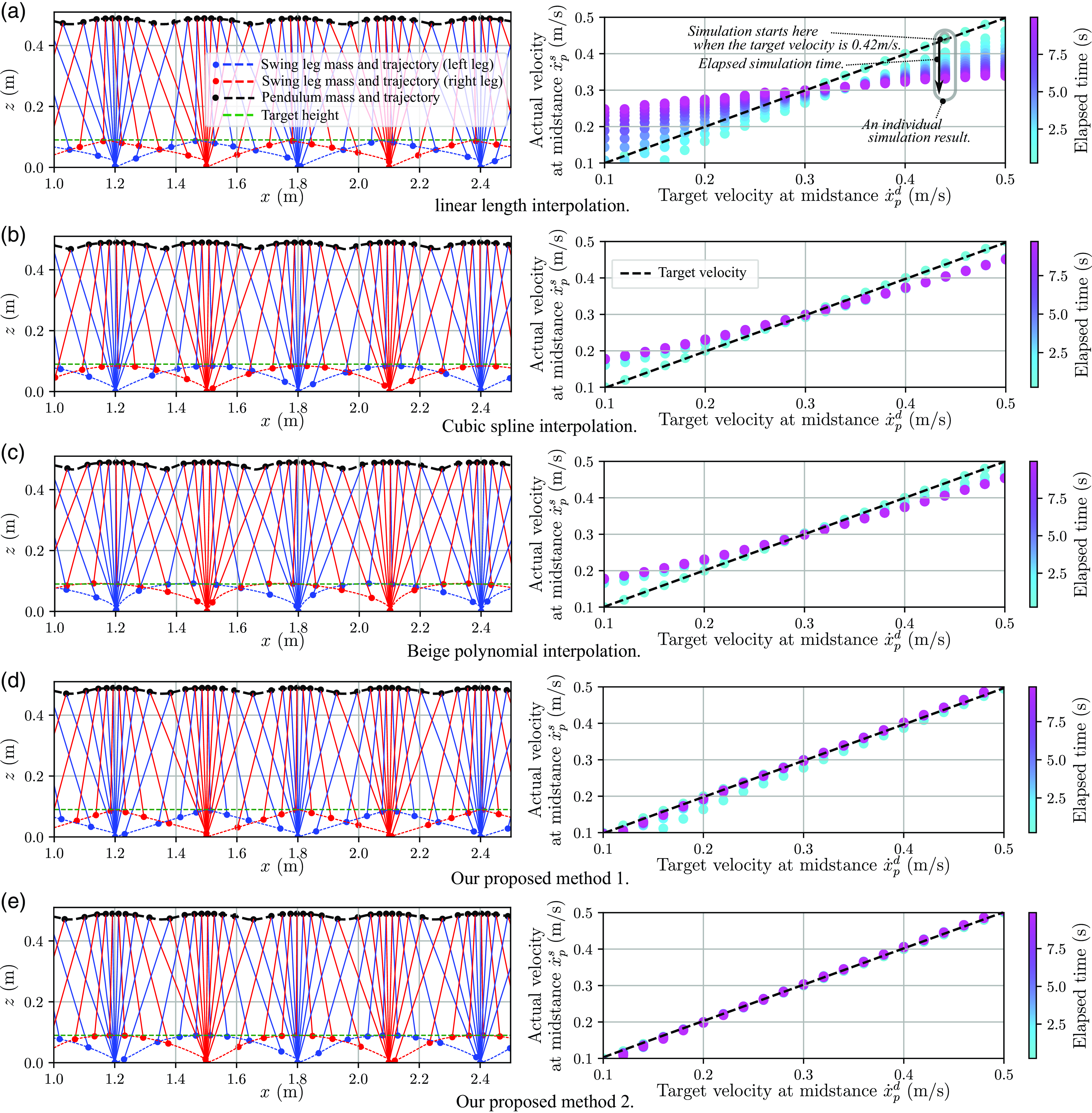
Figure 6. Trajectories of each mass for various swing-leg trajectory generation methods and the corresponding time-elapsed velocity changes. In the left diagrams of each panel, blue and red represent the trajectories of the left and right feet, respectively, while the green dashed line indicates the target height. In the right diagrams of each panel, the dashed line represents the target velocity, and the dots plot the observed velocity results. Note that the velocities converge near the purple region in each result. For simplicity, the CoM position of the swing leg is assumed to coincide with the foot position.
Additionally, Figure 7 illustrates the velocity trajectories for the linear length interpolation and proposed method 1, as shown in Figure 6. In Panel (a), the concave apex is intended to reach the dashed line at 0.2 m/s, which represents the target velocity for the simulation. While both methods begin from the same initial state, where the target and actual velocities are identical, the blue line gradually accelerates and diverges from the dashed line. In contrast, the proposed method (red line) remains close to the target velocity, periodically reaching it. Panels (b) and (c) display the phase diagrams of velocity for each method. The proposed method maintains a consistent velocity trajectory over time, whereas the linear length interpolation gradually transitions and converges to a trajectory distinct from the initial state.

Figure 7. Comparison of velocity trajectories. Panel (a) illustrates changes in forward velocity with and without the proposed method. Panels (b) and (c) present phase diagrams of forward and vertical velocities, respectively. The black dashed lines in all panels indicate the target velocity at the mid-stance position.
In this study, we compared our proposed method with other interpolation methods for swing-leg trajectories, focusing on whether intermittent control could effectively regulate the robot walking behavior in each approach. For methods other than the proposed method, significant velocity drift was observed. This indicates the presence of additional energy variations not accounted for by the motion and potential energy of the pendulum mass and swing-leg mass, which may potentially lead to unintended accelerations and decelerations caused by the swing-leg motion. To address this issue, it would be necessary to apply negative energy through upper body motions as feedback control during the SS phase. This approach aligns with existing methods using the LIP model [Reference Kim, Jorgensen, Lee, Ahn, Luo and Sentis18, Reference Kajita, Yamaura and Kobayashi14], which continuously compensates for momentum components to ensure the model adheres to its trajectory during the SS phase. However, such continuous feedback hinders this study’s primary goal, which is intermittently controlling the robot. In contrast, our proposed method provides a practical and effective solution, enabling intermittent control while addressing the limitations of existing approaches.
4.2. Velocity trackability evaluations by robot experiment
In the robot experiments, we verified that the proposed controller could track the target velocity in the dynamics simulator using Mujoco and actual hardware with our developed bipedal robot [Reference Kamioka, Shin, Yamaguchi and Muromachi15, Reference Kuo, Shin and Matsubara21], as shown in Figure 8. The bipedal robot has four degrees of freedom constrained to a two-dimensional plane. The conversion from the swing-leg trajectory to the robot is detailed in [Reference Kamioka, Shin, Yamaguchi and Muromachi15]. We measured the walking data of the robot for up to 10 footsteps in the simulation experiments and 6.5 m (approximately 20 footsteps) in the hardware experiments at each target velocity. In the simulation experiments, target velocities ranging from 0.10 to 0.50 m/s in increments of 0.05 m/s were given to the robot. In the hardware experiments, target velocities ranging from 0.10 to 0.50 m/s in increments of 0.20 m/s were used. The walking velocity for each step was measured as the average velocity at the midstance of the hip for
 $|\theta | \lt 0.005$
rad (depicted in Figure 1). The mean velocity at the midstance is represented as a dot, and the standard deviation is illustrated as a blue line. The results indicate that the average velocity successfully tracked the target velocity. Note that the standard deviation increased at lower speeds, which can be attributed to the difficulty of maintaining stability at very low walking speeds. This is because the controller parameters were tuned for a target velocity centered around 0.3 m/s, and the same parameters were used across all simulations. In the hardware experiments, the standard deviation was relatively large, likely due to the robot’s connected boom system, which generates characteristic vibrations. Nonetheless, the experimental results demonstrated that the average walking velocity converged to the target velocity.
$|\theta | \lt 0.005$
rad (depicted in Figure 1). The mean velocity at the midstance is represented as a dot, and the standard deviation is illustrated as a blue line. The results indicate that the average velocity successfully tracked the target velocity. Note that the standard deviation increased at lower speeds, which can be attributed to the difficulty of maintaining stability at very low walking speeds. This is because the controller parameters were tuned for a target velocity centered around 0.3 m/s, and the same parameters were used across all simulations. In the hardware experiments, the standard deviation was relatively large, likely due to the robot’s connected boom system, which generates characteristic vibrations. Nonetheless, the experimental results demonstrated that the average walking velocity converged to the target velocity.

Figure 8. The experimental results for velocity trackability with our bipedal robot with four degrees of freedom constrained in a two-dimensional plane. Panel (a) shows the dynamics simulator results, and panel (b) shows the hardware experiment results. The blue dots indicate the average velocities at the midstance, and the blue area represents the standard deviation. Panel (c) illustrates the progression of forward velocity when the target velocity is set to 0.3 m/s, and panel (d) depicts the trajectories of each mass during this condition. The blue circles represent the left foot, and the red circles represent the right foot. Panel (e) shows the stability verification results under external disturbances applied under the same conditions as panel (c). The upper part of the graph indicates the walking steps where external forces were applied to the pendulum mass: red numbers represent −10 N, and blue numbers represent + 10 N in the x-axis direction.
Figure 8 (c), (d), and (e) illustrates the velocity trajectory, CoM trajectories, and stability under external disturbances for the target velocity of 0.3 m/s shown in Panel (a). In Panel (c), it can be observed that the peak velocity reaches the target velocity indicated by the dashed line, repeatedly tracking it. Panel (d) depicts the corresponding trajectories, with the paths at the center of the graph and the circles representing the CoM trajectories of the legs. In swing phase (I), the trajectory forms an elliptical path, while in swing phase (II), it transitions to an ellipse resembling a straight line. These trajectories are determined by (10). Interestingly, the foot trajectory exhibits a characteristic path. This trajectory is not arbitrarily defined but rather emerges naturally due to the leg linkage mechanism when the swing-leg CoM follows an elliptical trajectory. Notably, this resembles the CoM trajectory observed in human walking, as described in [Reference Kitagawa and Ogihara19]. Lastly, Panel (e) demonstrates stability under external disturbances. External forces (+10 N or −10 N) were applied to the pendulum mass at specific timings during walking, as indicated by the red and blue numbers in Panel (e). These forces temporarily caused deviations from the target velocity, but once removed, the velocity consistently returned to the target value. The forces were applied multiple times, repeatedly testing the robot’s ability to recover to the target velocity, demonstrating sufficient stability for velocity tracking. This analysis highlights the stability of the proposed method under external disturbances, with consistent recovery observed regardless of the force direction.
5. Conclusion and future works
In this paper, we proposed an intermittent walking control method for the multi-mass model to control robot behavior by adjusting the energy during the DS phase and using zero-input control with a constrained swing-leg trajectory during the SS phase. The proposed method models the dynamics of a multi-mass system during the SS phase, including the swing-leg mass, as a conservative system. This allows the dynamical system to have a closed-form solution of the EoM, with behavior uniquely determined by the initial state. Furthermore, this modeling enables control of robot behavior with intermittent control inputs. The numerical simulation results demonstrated that the dynamical system of our proposed method is conservative. Both simulations and actual robot experiments confirmed that the proposed intermittent controller enables the robot to stabley track the target walking velocity. These results indicate that robot motion, including that of the multi-mass model, can be intermittently controlled by providing holonomic position constraints.
Through the numerical simulation, it was observed that the conserved energy changed discontinuously during the transition from phase (I) to phase (II), as shown by the blue line in Figure 6. While this discontinuity did not cause significant issues in the experiment, it evidences discontinuous acceleration of the swing leg. Therefore, developing a smoother method for phase transitions is anticipated.
In modeling the dynamics of the whole robot, the multi-mass model assumed in this paper adds additional masses to a pendulum mass. When more than two masses are added, their motions can influence one another depending on tracking performance. Developing a method to mitigate these influences is a research topic that will be researched further.
These extensions enable capturing a wide range of passive motions (zero-input control) before the passive motion begins, allowing various motions and robots to take advantage of intermittent controllers, which are energetically and computationally efficient. In the future, we aim to apply this method to three-dimensional humanoid robots with upper bodies.
Author contributions
HS, FC, and TK conceived and designed the study. TK developed the robot system. HS and TK developed the controller and hardware for the simulator. HS conducted the experiments, data gathering, and analyses. HS, FC, and TK wrote the article.
Financial support
This research received no specific grant from any funding agency, commercial, or not-for-profit sectors.
Competing interests
The authors declare no conflicts of interest exist.
Ethical approval
None.
A. Derivation of numerical simulation model
As shown in Figure 1(a), let the mass and the position of the pendulum mass model be
 $m_{p}$
and
$m_{p}$
and
 $\boldsymbol{p}_{p} = {x_{p}, z_{p}}^T$
, respectively. Then, the EoM for the double mass model is given by (2a). For the case in which the force
$\boldsymbol{p}_{p} = {x_{p}, z_{p}}^T$
, respectively. Then, the EoM for the double mass model is given by (2a). For the case in which the force
 $\boldsymbol{f}_{a}$
is applied at the additional mass position
$\boldsymbol{f}_{a}$
is applied at the additional mass position
 $\boldsymbol{p}_{a}$
, as shown in Figure 1(b), the external force
$\boldsymbol{p}_{a}$
, as shown in Figure 1(b), the external force
 $\boldsymbol{f}$
is calculated as the resultant of two forces:
$\boldsymbol{f}$
is calculated as the resultant of two forces:
 \begin{align} \boldsymbol{f} =\boldsymbol{f}_{r} + \boldsymbol{f}_{s}, \end{align}
where
 $\boldsymbol{f}_r$
is directly applied from
$\boldsymbol{f}_r$
is directly applied from
 $\boldsymbol{f}_{a}$
as shown in (7a). Assuming a spring mass model,
$\boldsymbol{f}_{a}$
as shown in (7a). Assuming a spring mass model,
 $\boldsymbol{f}_s$
is defined as follows:
$\boldsymbol{f}_s$
is defined as follows:
 \begin{eqnarray} \boldsymbol{f}_{s} = - k \boldsymbol{p}_{p} + C(\dot {\boldsymbol{p}}_{p},\boldsymbol{p}_{p}). \end{eqnarray}
The spring term is calculated as
 \begin{equation} k = \left \{ \begin{array}{ll} \boldsymbol{0} &\quad (|\boldsymbol{p}_{p}| \geq l) \\ k_0 \left ( 1 - \frac {l}{|\boldsymbol{p}_{p}|} \right ) &\quad (|\boldsymbol{p}_{p}| \lt l) \\ \end{array} \right ., \end{equation}
where
 $l = l_0 + l_f$
. The spring force can be adjusted by displacement of the spring’s natural length
$l = l_0 + l_f$
. The spring force can be adjusted by displacement of the spring’s natural length
 $l_f$
. In this model, the kick controller applies energy by adjusting the spring displacement
$l_f$
. In this model, the kick controller applies energy by adjusting the spring displacement
 $l_f$
. In addition, in order to add a damper in parallel to the spring in (A1), the following term is added to the right-hand side of (A2):
$l_f$
. In addition, in order to add a damper in parallel to the spring in (A1), the following term is added to the right-hand side of (A2):
 \begin{equation} C(\dot {\boldsymbol{p}}_{p},\boldsymbol{p}_{p}) = \left \{ \begin{array}{ll} 0 &\quad (|\boldsymbol{p}_{p}| \geq l) \\ -c_0\frac {\boldsymbol{p}_{p}^T{\dot {\boldsymbol{p}}_{p}}}{|\boldsymbol{p}_{p}|^2} \boldsymbol{p}_{p} &\quad (|\boldsymbol{p}_{p}| \lt l) \\ \end{array} \right . . \end{equation}
In the paper, a small damper is included to stabilize the simulation. In our numerical simulation explained in Section 4.1, the spring and damper constants are
 $k_0 = 10,000$
N/m and
$k_0 = 10,000$
N/m and
 $c_0 = 500$
Ns/m, respectively. The simulation numerically integrated (2a), (2b), (7a)
$c_0 = 500$
Ns/m, respectively. The simulation numerically integrated (2a), (2b), (7a)
 $\sim$
(7b), and (A1)
$\sim$
(7b), and (A1)
 $\sim$
(A4) using the Euler method.
$\sim$
(A4) using the Euler method.
The energy of the spring is calculated as follows:
 \begin{eqnarray} E_s = \frac {1}{2}\frac {( k \boldsymbol{p}_{p})^2}{k_0}. \end{eqnarray}
Note that we ignore the energy loss of the damper because the effect of the damper is small in our simulation.
B. Relationships used for algebraic manipulation
Assuming that a leg is an inverted pendulum with contacting foot to ground (i.e., Assumption1 and 3), the following deformations are derived:
 \begin{align} \dot {\boldsymbol{p}}_{p} = \dot {\boldsymbol \theta }_{p} \times \boldsymbol{p}_{p}, \;\;\; and \;\;\; l^2\dot {\boldsymbol \theta }_{p} = \boldsymbol{p}_{p} \times \dot {\boldsymbol{p}}_{p}. \end{align}
Following, we introduce transformation formulas related to the cross-product. The cross-product of the inner product of two matrices and the cross product can be obtained as follows:
 \begin{align} \boldsymbol{C}_{a} \boldsymbol{p}_{p} \times \boldsymbol{C}_{a} \ddot {\boldsymbol{p}}_{p} = \begin{cases} |\boldsymbol{C}_{a}| (\boldsymbol{p}_{p} \times \ddot {\boldsymbol{p}}_{p}) & (if \; 2D)\\ |\boldsymbol{C}_{a}| \boldsymbol{C}_{a}^{-T}(\boldsymbol{p}_{p} \times \ddot {\boldsymbol{p}}_{p}) & (if \; 3D)\end{cases}, \end{align}
 \begin{align} \boldsymbol{C}_{a} \boldsymbol{p}_{p} \times \boldsymbol{g} = \begin{cases} |\boldsymbol{C}_{a}| (\boldsymbol{p}_{p} \times \boldsymbol{C}_{a}^{-1} \boldsymbol{g}) & (if \; 2D)\\ |\boldsymbol{C}_{a}| \boldsymbol{C}_{a}^{-T}(\boldsymbol{p}_{p} \times \boldsymbol{C}_{a}^{-1} \boldsymbol{g}) & (if \; 3D) \end{cases}. \end{align}
These relationships are used for the derivative in the Appendix. D.
Note that we often use the following relation for antiderivative in Appendix D:
 \begin{align} \frac {1}{l^2} \int ( \boldsymbol{p}_{p} \times \ddot {\boldsymbol{p}}_{p} )^T (\boldsymbol{p}_{p}\times \dot {\boldsymbol{p}}_{p} ) dt & = \int ( \boldsymbol{p}_{p} \times \ddot {\boldsymbol{p}}_{p} )^T \dot {\boldsymbol \theta }_{p} dt = \int ( \dot {\boldsymbol \theta }_{p} \times \boldsymbol{p}_{p} )^T \ddot {\boldsymbol{p}}_{p} dt \notag \\ & = \int \dot {\boldsymbol{p}}_{p}^T \ddot {\boldsymbol{p}}_{p} dt = \frac {1}{2} \dot {\boldsymbol{p}}_{p}^T\dot {\boldsymbol{p}}_{p}. \end{align}
C. Derivation of energy: force component
When the constraint position trajector, such as (10) to the pendulum mass, is given to (9a), the following antiderivative, which is energy for the additional moment (7a), is obtained:
 \begin{equation} \begin{aligned} \int \boldsymbol{f}_{r}^T \dot {\boldsymbol{p}}_{p} dt &= -m_{a} \int (\ddot {\boldsymbol{p}}_{a} + \boldsymbol{g})^T \dot {\boldsymbol{p}}_{p} dt \\ &= -m_{a} \boldsymbol{g}^T \boldsymbol{p}_{p} - m_{a} \int \ddot {\boldsymbol{p}}_{a}^T \dot {\boldsymbol{p}}_{p} dt. \end{aligned} \end{equation}
D. Derivation of energy: moment component
When the constraint position trajectory, such as (10) to the pendulum mass, is given to (9a), the following antiderivative, which is energy for the additional force (7b), is obtained:
 \begin{align} \int \boldsymbol{\tau}_{r}^T \dot {\boldsymbol \theta }_{p} dt = & \int \frac {m_{a} }{l^2} \left ((\boldsymbol{p}_{p} - \boldsymbol{p}_{a} ) \times (\ddot {\boldsymbol{p}}_{a} + \boldsymbol{g})\right )^T (\boldsymbol{p}_{p}\times \dot {\boldsymbol{p}}_{p} ) dt \notag \\ = & \int \left (\frac {m_{a} }{l^2} \boldsymbol{p}_{p} \times \ddot {\boldsymbol{p}}_{a} \right )^T (\boldsymbol{p}_{p}\times \dot {\boldsymbol{p}}_{p} ) dt + \int \left (\frac {m_{a} }{l^2} \boldsymbol{p}_{p} \times \boldsymbol{g}\right )^T (\boldsymbol{p}_{p}\times \dot {\boldsymbol{p}}_{p} ) dt \notag \\ & - \int \left (\frac {m_{a} }{l^2} \boldsymbol{p}_{a} \times \ddot {\boldsymbol{p}}_{a} \right )^T (\boldsymbol{p}_{p}\times \dot {\boldsymbol{p}}_{p} ) dt - \int \left (\frac {m_{a} }{l^2} \boldsymbol{p}_{a} \times \boldsymbol{g} \right )^T (\boldsymbol{p}_{p}\times \dot {\boldsymbol{p}}_{p} ) dt. \end{align}
Using the manipulations and relations (B1)
 $\sim$
(B3), the right-hand side of (D1) is extended as follows:
$\sim$
(B3), the right-hand side of (D1) is extended as follows:
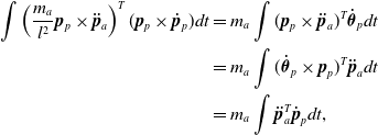 \begin{align} \qquad \int \left (\frac {m_{a} }{l^2} \boldsymbol{p}_{p} \times \ddot {\boldsymbol{p}}_{a} \right )^T (\boldsymbol{p}_{p}\times \dot {\boldsymbol{p}}_{p} ) dt &= m_{a} \int (\boldsymbol{p}_{p} \times \ddot {\boldsymbol{p}}_{a} )^T \dot {\boldsymbol \theta }_{p} dt \notag \\ &= m_{a} \int (\dot {\boldsymbol \theta }_{p} \times \boldsymbol{p}_{p} )^T \ddot {\boldsymbol{p}}_{a} dt \notag \\ &= m_{a} \int \ddot {\boldsymbol{p}}_{a}^T \dot {\boldsymbol{p}}_{p} dt, & \end{align}
 \begin{align} \qquad \int \left (\frac {m_{a} }{l^2} \boldsymbol{p}_{p} \times \boldsymbol{g} \;\;\right )^T (\boldsymbol{p}_{p}\times \dot {\boldsymbol{p}}_{p} ) dt &= m_{a} \int (\boldsymbol{p}_{p} \times \boldsymbol{g} )^T \dot {\boldsymbol \theta }_{p} dt \notag \\ &= m_{a} \int (\dot {\boldsymbol \theta }_{p} \times \boldsymbol{p}_{p} )^T \boldsymbol{g} dt \notag \\ &= m_{a} \boldsymbol{g}^T \boldsymbol{p}_{p}, & \end{align}
 \begin{align} \qquad \int \left (\frac {m_{a}}{l^2} \boldsymbol{p}_{a} \times \ddot {\boldsymbol{p}}_{a} \right )^T (\boldsymbol{p}_{p}\times \dot {\boldsymbol{p}}_{p} ) dt \notag &= \frac {m_{a} }{l^2} \int (\boldsymbol{B}_{a} \times \ddot {\boldsymbol{p}}_{a} )^T (\boldsymbol{p}_{p}\times \dot {\boldsymbol{p}}_{p} ) dt + \frac {m_{a} }{l^2} \int (\boldsymbol{C}_{a} \boldsymbol{p}_{p} \times \boldsymbol{C}_{a} \ddot {\boldsymbol{p}}_{p} )^T(\boldsymbol{p}_{p}\times \dot {\boldsymbol{p}}_{p} ) dt \notag \\ &= m_{a} \int ( \boldsymbol{B}_{a} \times \ddot {\boldsymbol{p}}_{p} )^T \dot {\boldsymbol \theta }_{p} dt + \begin{cases} \frac {1}{2}m_{a} |\boldsymbol{C}_{a} | \dot {\boldsymbol{p}}_{p}^T \dot {\boldsymbol{p}}_{p} & (if \; 2D) \\ \frac {1}{2}m_{a} |\boldsymbol{C}_{a}| \boldsymbol{C}_{a}^{-T} \dot {\boldsymbol{p}}_{p}^T \dot {\boldsymbol{p}}_{p} & (if \; 3D) \end{cases}, & \end{align}
 \begin{align} \qquad \int \left (\frac {m_{a} }{l^2} \ddot {\boldsymbol{p}}_{a} \times \boldsymbol{g} \right )^T (\boldsymbol{p}_{p}\times \dot {\boldsymbol{p}}_{p} ) dt &= m_{a} \int (\boldsymbol{B}_{a}\times \boldsymbol{g})^T\dot {\boldsymbol \theta }_{p} dt + m_{a} \int (\boldsymbol{C}_{a} \boldsymbol{p}_{p} \times \boldsymbol{g} )^T \dot {\boldsymbol \theta }_{p} dt \notag \\ &= m_{a} (\boldsymbol{B}_{a}\times \boldsymbol{g})^T \boldsymbol{\theta }_{p} + \begin{cases} \int m_{a} |\boldsymbol{C}_{a}| (\boldsymbol{p}_{p} \times \boldsymbol{C}_{a}^{-1}\boldsymbol{g} )^T \dot {\boldsymbol \theta }_{p} dt & (if \; 2D)\\ \int m_{a} |\boldsymbol{C}_{a}| \boldsymbol{C}_{a}^{-T} (\boldsymbol{p}_{p} \times \boldsymbol{C}_{a}^{-1}\boldsymbol{g} )^T \dot {\boldsymbol \theta }_{p} dt & (if \; 3D) \end{cases} \notag \\ &= m_{a} (\boldsymbol{B}_{a}\times \boldsymbol{g})^T \boldsymbol{\theta }_{p} + \begin{cases} \int m_{a} (|\boldsymbol{C}_{a}| \boldsymbol{C}_{a}^{-1}\boldsymbol{g})^T (\dot {\boldsymbol \theta }_{p} \times \boldsymbol{p}_{p} ) dt & (if \; 2D)\\ \int m_{a} (|\boldsymbol{C}_{a}| \boldsymbol{C}_{a}^{T} \boldsymbol{g})^T (\dot {\boldsymbol \theta }_{p} \times \boldsymbol{p}_{p} ) dt & (if \; 3D) \end{cases} \notag \\ &= m_{a} (\boldsymbol{B}_{a}\times \boldsymbol{g})^T \boldsymbol{\theta }_{p} + \begin{cases} m_{a} \left (|\boldsymbol{C}_{a}|\boldsymbol{C}_{a}^{-1} \boldsymbol{g} \right )^T \boldsymbol{p}_{p} & (if \; 2D)\\ m_{a} \left (|\boldsymbol{C}_{a}|\boldsymbol{C}_{a}^{-T} \boldsymbol{g} \right )^T \boldsymbol{p}_{p} & (if \; 3D) \end{cases}. & \end{align}
E. Sum of total additional energy
From derivation as shown in Appendix C and D, the sum of total additional energy (9a) is obtained as follows:
 \begin{align} \int \boldsymbol{f}_{r}^T \dot {\boldsymbol{p}}_{p} dt + \int \boldsymbol{\tau}_{r}^T \dot {\boldsymbol \theta }_{p} dt &= - \frac {1}{2}m_{a} |\boldsymbol{C}_{a} | \dot {\boldsymbol{p}}_{p}^T \dot {\boldsymbol{p}}_{p} - m_{a} \left (|\boldsymbol{C}_{a}|\boldsymbol{C}_{a}^{-1} \boldsymbol{g} \right )^T \boldsymbol{p}_{p} \notag \\ &- m_{a} (\boldsymbol{B}_{a}\times \boldsymbol{g})^T \boldsymbol{\theta }_{p} - m_{a} \int ( \boldsymbol{B}_{a} \times \ddot {\boldsymbol{p}}_{p} )^T \dot {\boldsymbol \theta }_{p} dt. \end{align}
The parameter of the remaining term, which cannot be integrated, is relatively small compared to other parameters and can be ignored, allowing the system to assume an approximate conservative system. Especially, when
 $\boldsymbol{B}_{a} = \{0, b_z\}$
,
$\boldsymbol{B}_{a} = \{0, b_z\}$
,
 $\boldsymbol{B}_{a}$
and
$\boldsymbol{B}_{a}$
and
 $\ddot {\boldsymbol{p}}_{p}$
are almost in the same direction because
$\ddot {\boldsymbol{p}}_{p}$
are almost in the same direction because
 $\boldsymbol{p}_{p}$
follows a circular motion. As a result,
$\boldsymbol{p}_{p}$
follows a circular motion. As a result,
 $\boldsymbol{B}_{a} \times \ddot {\boldsymbol{p}}_{p}$
can be approximated as nearly zero. Then, the sum of energy can be obtained with a small approximation as follows:
$\boldsymbol{B}_{a} \times \ddot {\boldsymbol{p}}_{p}$
can be approximated as nearly zero. Then, the sum of energy can be obtained with a small approximation as follows:
 \begin{align} \int \boldsymbol{f}_{r}^T \dot {\boldsymbol{p}}_{p} dt + \int \boldsymbol{\tau}_{r}^T \dot {\boldsymbol \theta }_{p} dt &\simeq - \frac {1}{2}m_{a} |\boldsymbol{C}_{a} | \dot {\boldsymbol{p}}_{p}^T \dot {\boldsymbol{p}}_{p} - m_{a} \left (|\boldsymbol{C}_{a}|\boldsymbol{C}_{a}^{-1} \boldsymbol{g} \right )^T \boldsymbol{p}_{p} - m_{a} (\boldsymbol{B}_{a}\times \boldsymbol{g})^T \boldsymbol{\theta }_{p}. \end{align}
On the other hand, the remaining term includes
 $\boldsymbol{B}_{a}$
. Furthermore, (10) has redundant parameters for obtaining a curve connecting two points. Therefore, we can give an arbitrary trajectory with
$\boldsymbol{B}_{a}$
. Furthermore, (10) has redundant parameters for obtaining a curve connecting two points. Therefore, we can give an arbitrary trajectory with
 $\boldsymbol{B}_{a} = \boldsymbol{0}$
. When
$\boldsymbol{B}_{a} = \boldsymbol{0}$
. When
 $\boldsymbol{B}_{a} = \boldsymbol{0}$
, the sum of energy is obtained as follows without approximation:
$\boldsymbol{B}_{a} = \boldsymbol{0}$
, the sum of energy is obtained as follows without approximation:
 \begin{align} \int \boldsymbol{f}_{r}^T \dot {\boldsymbol{p}}_{p} dt + \int \boldsymbol{\tau}_{r}^T \dot {\boldsymbol \theta }_{p} dt &= - \frac {1}{2}m_{a} |\boldsymbol{C}_{a} | \dot {\boldsymbol{p}}_{p}^T \dot {\boldsymbol{p}}_{p} - m_{a} \left (|\boldsymbol{C}_{a}|\boldsymbol{C}_{a}^{-1} \boldsymbol{g} \right )^T \boldsymbol{p}_{p}. \end{align}
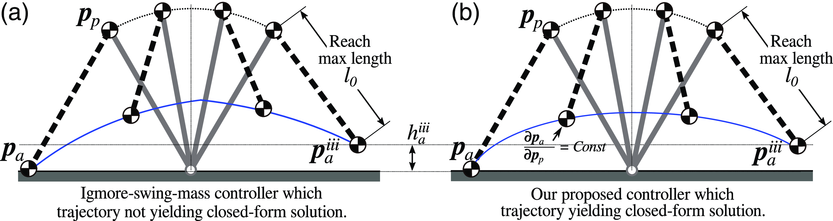
Figure 9. Swing-leg trajectories that show the comparative method and our method, respectively.
F. Generation of comparative swing trajectory
This section describes a method for generating a swing trajectory that is used for comparison with the swing trajectory (10) of the proposed controller. We refer to this as the ”ignore-swing-mass trajectory.” In order to make the velocity of the swing-leg mass position vary with walking velocity even if the target walking velocity is changed and to linearly change the x-position and swing-leg length depending on the pendulum mass posture, the ignore-swing-mass trajectory is given as follows:
 \begin{eqnarray} &&x_{a}^{\textrm { cmd}} = \left (1+K_{\textrm { ratio}}\right ) \left (x_{p}^{s}-x_{p}^{i}\right ) + x_{a}^{i}, \end{eqnarray}
 \begin{eqnarray} &&l_{\textrm { swg}}^{\textrm { cmd}} = \left (l_{\textrm { swx}}^{\textrm { max}}-l_{\textrm { swg}}^{\textrm { min}}\right ) \left | x_{p}^{s}-x_{s}^{\textrm { cmd}}\right | / \left |x_{p}^{s}-x_{val} \right | + l_{a}^{\textrm { min}}. \end{eqnarray}
When
 $x^{\textrm { cmd}}{a} \leq x{p}^{s}$
,
$x^{\textrm { cmd}}{a} \leq x{p}^{s}$
,
 $x_{val} = x_{a}^{i}$
. When
$x_{val} = x_{a}^{i}$
. When
 $x^{\textrm { cmd}}{a} \geq x{p}^{s}$
,
$x^{\textrm { cmd}}{a} \geq x{p}^{s}$
,
 $x_{val} = x_{a}^{d}$
. In the simulation, we defined
$x_{val} = x_{a}^{d}$
. In the simulation, we defined
 $x_{a}^{d} = x_{p}^{s} + 0.25$
. Moreover, when
$x_{a}^{d} = x_{p}^{s} + 0.25$
. Moreover, when
 $x^{\textrm { cmd}}{a} \geq x{p}^{s}$
and
$x^{\textrm { cmd}}{a} \geq x{p}^{s}$
and
 $l_{a}^{\textrm { cmd}} \geq l_{a}^{\textrm { max}}$
, we set
$l_{a}^{\textrm { cmd}} \geq l_{a}^{\textrm { max}}$
, we set
 $l_{a}^{\textrm { cmd}} = l_{a}^{\textrm { max}}$
. Then, the leg length control stops when the leg length exceeds the maximum length (natural length of the springs). By changing
$l_{a}^{\textrm { cmd}} = l_{a}^{\textrm { max}}$
. Then, the leg length control stops when the leg length exceeds the maximum length (natural length of the springs). By changing
 $K_{\textrm { ratio}}$
, the position at which the leg length control stops can be adjusted. In our simulation, to ensure that the ignore-swing-mass trajectory has the same swing end clearance as the proposed controller, we used
$K_{\textrm { ratio}}$
, the position at which the leg length control stops can be adjusted. In our simulation, to ensure that the ignore-swing-mass trajectory has the same swing end clearance as the proposed controller, we used
 $l_{a}^{\textrm { min}} = 0.40$
,
$l_{a}^{\textrm { min}} = 0.40$
,
 $l_{a}^{\textrm { max}} = 0.50$
, and
$l_{a}^{\textrm { max}} = 0.50$
, and
 $K_{\textrm { ratio}} = 1.65$
.
$K_{\textrm { ratio}} = 1.65$
.
G. Verification Results with Different Parameters
Figure 10 shows the results of the parameter variation experiments, based on the comparative verification test in the main text (Figs. 6(d) and (e)). Panel (a) presents the results with modified parameters in the forward direction, while panel (b) shows the results with modified parameters in the vertical direction. Note that, for panel (a), the trajectory generation method from Figure 6(d) was used to make the changes in the forward direction more comprehensible. apart from the parameters shown in the figure, all other parameters remained unchanged. Both results confirm accurate tracking of the target velocity.

Figure 10. Numerical simulation results with different parameters compared to Figure 6(d) and (e).


