


1. Introduction
In the field of control systems, optimal control theory is a key approach for addressing the degrees of freedom problem. This involves defining an objective function and finding its extremum under the constraints of the system’s equations of motion and allowable control variables. A substantial body of literature has explored various objective functions, including minimising the square of the hand’s jerk over an entire movement [Reference Morasso1], integrated torque change [Reference Uno, Kawato and Suzuki2], minimum object crackle [Reference Dingwell, Mah and Mussa-Ivaldi3], and minimum acceleration criterion [Reference Ben-Itzhak and Karniel4]. Despite these advances, a significant challenge remains in deriving optimal solutions for nonlinear time-varying systems, especially as the complexity of the objective function and constraints increases. The mathematical process of computing the optimal feedback controller in such cases is notably intricate [Reference Scott5]. While evolutionary algorithms offer a promising method for addressing these challenges [Reference Zeidler, Frey, Kompa and Motzkus6,Reference Diveev, Sofronova and Konstantinov7], they are often limited by the risk of converging to local optima rather than global solutions.
In robotics, generating complex motor behaviours that rival human capabilities remains a significant challenge [Reference Billard and Kragic8]. For instance, to enhance the performance of human–robot cooperation tasks, a system where the human arm grasps a robot handle has been modelled as a closed kinematic chain, evaluated using ergonomics-related criteria [Reference Sharkawy9]. This approach improves human–robot interaction by increasing accuracy, stability, and user comfort, but it often comes at the cost of task speed and completion time.
Rich, accurate, and stable motor behaviour can be understood as a sequence or superposition of fundamental motor primitives. Two distinct approaches [Reference Nah, Lachner and Hogan10] have been proposed to achieve this: dynamic movement primitives (DMPs), which consist of a canonical system, nonlinear forcing terms, and transformation systems [Reference Schaal11–Reference Saveriano, Abu-Dakka, Kramberger and Peternel13], and elementary dynamic actions (EDAs), which are based on submovements, oscillations, and mechanical impedance [Reference Hogan and Sternad14–Reference Hogan16].
The key differences between DMPs and EDAs are noteworthy. DMPs offer high-precision tracking using inverse dynamics but require an accurate robot model. In contrast, EDAs are better suited for managing uncertainties, as they do not rely on an inverse dynamics model. Instead, they use mechanical impedance to handle physical interactions and tracking errors. This paper explores and presents an EDAs-based approach, integrating impedance control, the passive motion paradigm (PMP) [Reference Mussa-Ivaldi, Morasso and Zaccaria17], and deep neural networks to control the manipulator’s end-effector. This approach addresses kinematic redundancy without solving the inverse kinematics problem, using deep neural networks to approximate kinematic transformations with reasonable accuracy.
Specifically, impedance control was developed to account for the mechanics of interactions between physical systems [Reference Hogan18]. Given that manipulation is inherently a nonlinear problem, it is crucial to distinguish between impedance and admittance; specifically, when interacting with inertial objects in the environment, the manipulator should be an impedance. To adapt the objective function of optimal control theory to the force field paradigm in impedance control, a neural network implementation [Reference Mohan and Morasso19] of the PMP has been developed for robot manipulation, based on the equilibrium point hypothesis [Reference Bizzi, Hogan, Mussa-Ivaldi and Giszter20]. This process can qualitatively represent how the brain allocates work across a redundant set of joints when the end-effector is tasked with reaching a specific point in space. It is described as an “internal simulation process”, calculating the movement of each joint if an external force (i.e., the goal) were to draw the end-effector slightly towards the target. The term “passive” aligns with the equilibrium point hypothesis, suggesting that the brain does not explicitly determine the equilibrium point but instead contributes to the activation of “task-related” force fields [Reference Mohan, Bhat and Morasso21]. To date, the PMP model has been applied in various contexts, including combining postural and focal synergies during whole-body reaching tasks [Reference Morasso, Casadio, Mohan and Zenzeri22], coordinating the movements of a humanoid robot’s upper body and a paintbrush to generate motor commands for drawing shapes [Reference Mohan, Morasso, Zenzeri, Metta, Chakravarthy and Sandini23], and developing the Pinocchio framework for action representation using force fields [Reference Morasso and Mohan24]. Additionally, this model has also been utilised in an agricultural robot to control a manipulator for harvesting soft fruit [Reference Wang, Urquizo, Roberts, Mohan, Newenham, Ivanov and Dowling25].
Implementing this model requires the Jacobian matrix of the kinematic mapping from joint angles to the end-effector position, which can be learnt through “babbling” movements and represented using artificial neural networks (ANNs) [Reference Mohan and Morasso26]. This method is similar to physics-informed neural networks, which incorporate physical laws—expressed as partial differential equations or other mathematical models—directly into the learning process [Reference Raissi, Perdikaris and Karniadakis27]. The Jacobian matrix, being a matrix of first-order partial derivatives arranged in a specific way, can be solved using this physics-informed neural network approach, i.e., by fitting the relationship between the joint angles and the end positions using the trained neural network weights for evaluation. ANNs make the kinematic model more flexible and adaptable to different configurations or robots with slightly varying link lengths or joint properties. This flexibility becomes useful when deploying the system across different manipulators with minimal adjustments.
Although this method is theoretically feasible, it demands a large amount of data and considerable computing time for training to obtain an accurate and effective Jacobian matrix. Moreover, ANNs are prone to overfitting. Additionally, the results of each training session are specific to one kinematic parameter of the manipulator, necessitating the retraining of new ANN parameters if the model is to be deployed on different manipulators.
To address the concerns mentioned above, this study first investigates the influence of activation functions and network depth on ANN training performance for these “babbling” movements. With advancements in deep learning, PMP models based on deep neural networks have been developed to overcome the limitations of traditional ANNs. Furthermore, this paper explores the use of transfer learning [Reference Pan and Yang28] to improve the transferability and adaptability of the PMP model across different manipulators. The enhanced model was validated on Universal Robots (UR arms), demonstrating its effectiveness. Additionally, we compared our method with MoveIt [Reference Sucan, Chitta and Contributors29] and Robotics Toolbox [Reference Corke and Haviland30], two widely used open-source motion planning frameworks in robotics. MoveIt typically employs motion planning approaches to solve inverse kinematics, yielding highly accurate results. In contrast, the PMP approach proposed here provides an EDAs-based method that balances reasonable accuracy with the inherent characteristics of EDAs. The Robotics Toolbox is used to develop a non-ANN-based PMP, compared with the ANN-based PMP. The code of ANN-based approximate kinematic transformations and PMP implementation are available at https://github.com/Fuli-Wang/Passive-motion-paradigm-implementation-via-ANN.git. Note: A summary of the symbols used in this paper can be found in Table I.
Table I. Table of symbols.

2. Problem statement
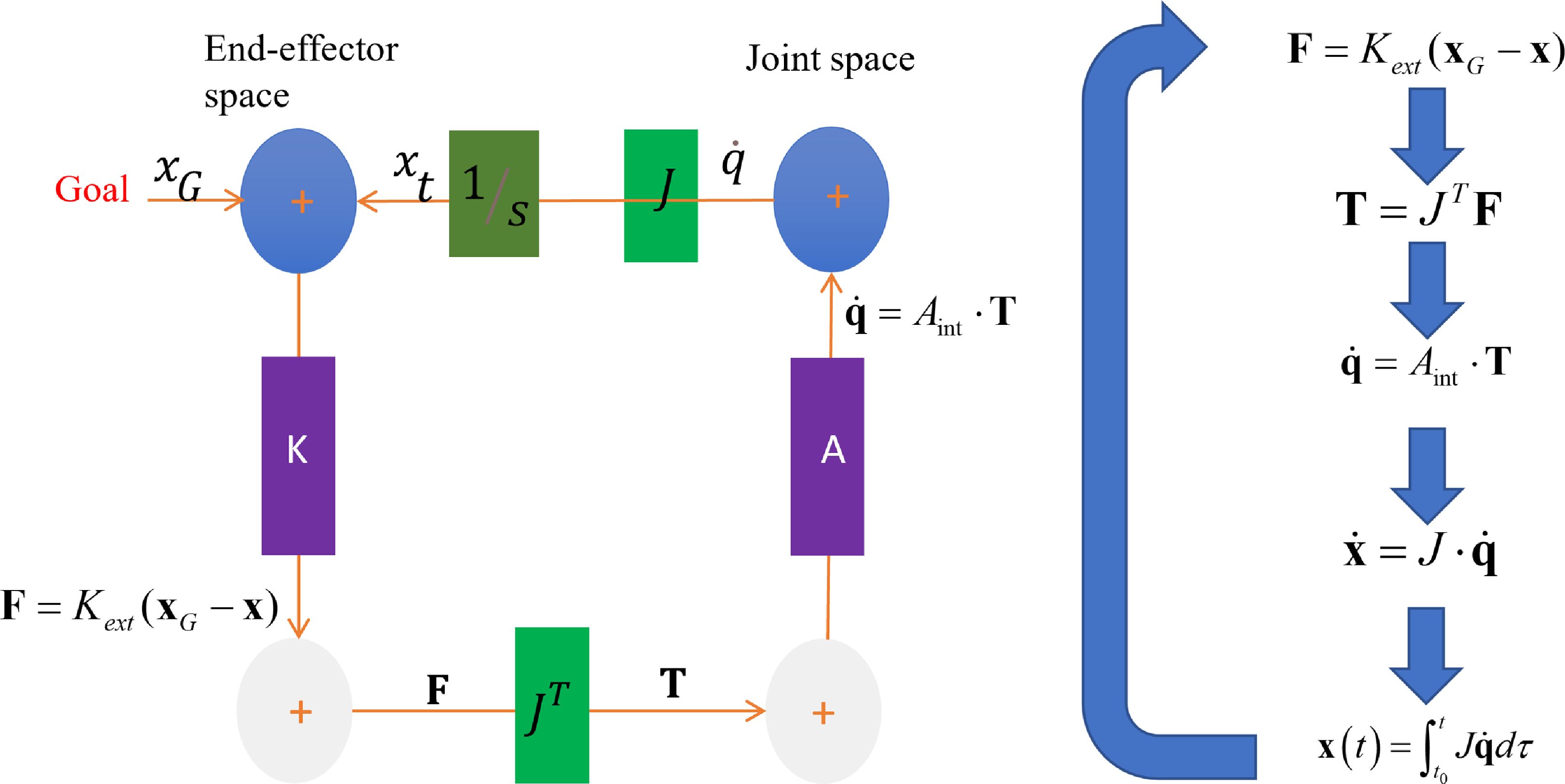
Figure 1. Basic kinematic network implements the passive motion paradigm for a simple kinematic chain (K: Stiffness, A: Admittance). As the end-effector gets closer to the goal, the virtual force tends to zero (equilibrium).
2.1. Implementation of impedance control
For the impedance control of manipulators, mathematically, the actuator is assumed to generate the commanded torque
 $ \mathbf {T}$
with the actuator angle
$ \mathbf {T}$
with the actuator angle
 $ \theta$
, and a kinematic relationship between the actuator angle and the end-point exists such that
$ \theta$
, and a kinematic relationship between the actuator angle and the end-point exists such that
 $ \mathbf {x} = \mathbf {L}(\theta )$
. Designing a feedback control law that coordinates the desired relationship between end-point force
$ \mathbf {x} = \mathbf {L}(\theta )$
. Designing a feedback control law that coordinates the desired relationship between end-point force
 $ \mathbf {F}$
and position
$ \mathbf {F}$
and position
 $ \mathbf {x}$
for implementation in an actuator is straightforward. To define the desired equilibrium position for the end-point without environmental forces as
$ \mathbf {x}$
for implementation in an actuator is straightforward. To define the desired equilibrium position for the end-point without environmental forces as
 $ \mathbf {x}_0$
, a general form for the desired force–position relation is
$ \mathbf {x}_0$
, a general form for the desired force–position relation is
 \begin{equation} \mathbf {F} = \mathbf {K}(\mathbf {x}_0 - \mathbf {x}) \end{equation}
According to the Jacobian matrix
 $ \mathbf {J}$
and the principle of virtual work, the required relationship in actuator coordinates is
$ \mathbf {J}$
and the principle of virtual work, the required relationship in actuator coordinates is
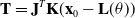 \begin{equation} \mathbf {T} = \mathbf {J}^T\mathbf {K}(\mathbf {x}_0 - \mathbf {L}(\theta )) \end{equation}
The relation
 $ \mathbf {K}(\mathbf {x}_0 - \mathbf {x})$
does not present any linear restrictions. The selected relation making the end-point stiff accomplishes Cartesian end-point position control and eliminates the inverse kinematics problem; only the forward kinematic equations for the manipulator must be computed.
$ \mathbf {K}(\mathbf {x}_0 - \mathbf {x})$
does not present any linear restrictions. The selected relation making the end-point stiff accomplishes Cartesian end-point position control and eliminates the inverse kinematics problem; only the forward kinematic equations for the manipulator must be computed.
2.2. Implementation of the PMP
Based on the impedance control theory, as shown in Figure 1 the PMP animation for a serial kinematic chain can be constructed to enable goal-directed actions. The equations used in this section are derived from biomechanics and robotics that focus on passive dynamics and control theory [Reference Hogan18,Reference Flash and Hogan31,Reference Spong, Hutchinson and Vidyasagar32] and the steps are as follows.
-
• This approach aligns closely with the EDAs framework, as described in ref. [Reference Nah, Lachner and Hogan10] how the robot interacts with its environment by specifying desired dynamics, like a desired force to achieve a goal position:
(3)where \begin{equation} \mathbf {F}_{\text {extr}} = \mathbf {K} (\mathbf {x}_G - \mathbf {x}) \end{equation}
$ \mathbf {x}_G$
denotes the goal to reach, and
$ \mathbf {K}$
is the virtual stiffness of the attractive field in the extrinsic space.
$ \mathbf {K}$
determines the shape and intensity of the force field. In the simplest case,
$ \mathbf {K}$
is proportional to an identity matrix, corresponding to an isotropic field converging to the target along straight flow lines. In line with the EDAs framework, this force generation serves as a primitive action that drives the movement towards the desired target.
\begin{equation} \mathbf {F}_{\text {extr}} = \mathbf {K} (\mathbf {x}_G - \mathbf {x}) \end{equation}
$ \mathbf {x}_G$
denotes the goal to reach, and
$ \mathbf {K}$
is the virtual stiffness of the attractive field in the extrinsic space.
$ \mathbf {K}$
determines the shape and intensity of the force field. In the simplest case,
$ \mathbf {K}$
is proportional to an identity matrix, corresponding to an isotropic field converging to the target along straight flow lines. In line with the EDAs framework, this force generation serves as a primitive action that drives the movement towards the desired target.
-
• Map the force field from the extrinsic space into the virtual torque field in the intrinsic space:
(4)This transformation aligns with the idea of EDAs, where motor commands are generated by mapping external forces into joint torques, thus allowing for a dynamic and adaptive response in the intrinsic space of the manipulator.
\begin{equation} \mathbf {T}_{\text {virt}} = \mathbf {J}^T \mathbf {F}_{\text {extr}} \end{equation}
-
• Relax the arm configuration to the applied field:
(5)where
\begin{equation} \dot {\mathbf {\theta }} = \mathbf {A} \mathbf {T}_{\text {virt}} \end{equation}
$ \mathbf {A}$
denotes the virtual admittance matrix in the intrinsic space. The modulation of this matrix affects the relative contributions of the different joints to the overall reaching movement. This control law helps the robot to adjust its motion and reach the position passively by controlling the stiffness and admittance of the system.
-
• Map the arm movement into the extrinsic workspace:
(6)This step integrates the motor primitive back into the extrinsic space, ensuring that the end-effector’s movement is dynamically coordinated with joint space behaviour, similar to the concept of EDAs synchronizing joint actions with overall task objectives.
\begin{equation} \dot {\mathbf {x}} = \mathbf {J} \dot {\mathbf {\theta }} \end{equation}
-
• Integrate over time until equilibrium:
(7)This step is integration, which provides a trajectory with the equilibrium configuration
\begin{equation} \mathbf {x}(t) = \int _{t_0}^{t} \mathbf {J} \dot {\mathbf {\theta }} d\tau \end{equation}
$ \mathbf {x}(t)$
defining the final position of the robot in the extrinsic space. All the computations in the above loop are “well-posed” and the relaxation mechanism does not require any objective function to solve the indeterminacy related to the excess redundancy problem. Time can be explicitly controlled by inserting a time-varying gain
$ \Gamma (t)$
in the nonlinear dynamics of the relaxation process (Eqs. 3–6). To achieve this, the technique originally proposed in [Reference Zak33] for content-addressable memories can be extended in the context of goal-directed reaching for robots [Reference Bhat, Akkaladevi, Mohan, Eitzinger and Morasso34].


This can be implemented by substituting the relaxation Eq. (5) with:
 \begin{equation} \dot {\mathbf {\theta }} = \Gamma (t) \mathbf {A} \mathbf {T}_{\text {virt}} \end{equation}
where a possible form of the time-varying gain is given by a minimum-jerk generator with duration
 $ t$
:
$ t$
:
 \begin{equation} \Gamma (t) = \frac {\xi (t)}{1 - \xi (t)} \end{equation}
where
 \begin{equation} \xi (t) = 6 \left (\frac {t}{\tau }\right )^5 - 15 \left (\frac {t}{\tau }\right )^4 + 10 \left (\frac {t}{\tau }\right )^3 \end{equation}
In general, a time-based generator can be used as a computational tool for synchronising multiple relaxations in composite PMP networks, essentially coordinating the relaxation of movements of two manipulators or even the body movements of humanoid robots. This concept reflects the EDAs principle of coordinating multiple primitive actions for complex, goal-directed behaviours.
For a simple reaching task with a manipulator, at the end of the animation process, four sets of trajectories are obtained as a function of time:
-
1. Sequence of joint angles given by the positioning node in the joint space.
-
2. Resulting consequence, i.e., the sequence of end-effector position in end-effector space.
-
3. Sequence of torques at the different joints in the joint space.
-
4. Resulting consequence, i.e., the sequence of forces applied by the end-effector in the end-effector space.
The time-varying gain is considered a temporal pressure that becomes stronger as the deadline approaches and diverges afterwards. Further details of the mathematical model for terminal attractor dynamics applied to goal-directed reaching in robots can be found in ref. [Reference Bhat, Akkaladevi, Mohan, Eitzinger and Morasso34].
Simultaneously, a range of internal and external constraints can be integrated at runtime based on the requirements of the task that needs to be performed, using force fields defined either in the extrinsic space or in the intrinsic space. Importantly, the Jacobian matrix in the PMP model characterises the kinematic properties of the manipulator. By importing the corresponding Jacobian matrix, it is possible to switch between PMP models for different manipulators.

Figure 2. Multi-layer perceptrons. The input is the angles of the six joints (assuming 6 degrees of freedom robotic arm), whereas the output is the 3D coordinate point of the end-effector. The network is trained to approximate the kinematic transformation and used to evaluate the Jacobian matrix. In the hidden layers, the tanh, sigmoid or relu functions are usually used as activation functions, but in the last layer, the linear function is used to let the coordinate values lie between positive infinity and negative infinity.
3. ANN-based approximate kinematic transformations
To approximate kinematic transformations using ANNs, data are typically obtained through sensorimotor exploration. In the manipulator’s workspace, joint rotation readings and corresponding end-effector coordinates are recorded based on forward kinematic analysis.
To illustrate a common ANN’s structure, as shown in Figure 2, PMPs are often based on this type of neural network to approximate motion transformations, i.e., two- or three-layer networks consisting of a number of neurons. With the increase in the number of layers and neurons to form deep neural networks, the general mathematical derivation of the Jacobian matrix based on the training weights is outlined below.
Consider a neural network with
 $ L$
layers. Let:
$ L$
layers. Let:
-
•
$ \theta \in \mathbb {R}^{n}$
be the input vector representing the joint angles. -
•
$ x \in \mathbb {R}^{3}$
be the output vector representing the end-effector 3D coordinates. -
•
$ W^{[l]}, b^{[l]}$
be the weights and biases for layer
$ l$
. -
•
$ f^{[l]}$
be the activation function for layer
$ l$
.


Forward Propagation
The forward propagation for each layer
 $ l$
is given by
$ l$
is given by
 \begin{equation} h^{[l]} = W^{[l]} z^{[l-1]} + b^{[l]}, \quad z^{[l]} = f^{[l]}(h^{[l]}) \quad \text {for } l = 1, \ldots, L \end{equation}
The final layer output is
 \begin{equation} x = W^{[L]} z^{[L-1]} + b^{[L]} \end{equation}
Jacobian Calculation
The Jacobian
 $ J \in \mathbb {R}^{3 \times n}$
of the output
$ J \in \mathbb {R}^{3 \times n}$
of the output
 $ x$
with respect to the input
$ x$
with respect to the input
 $ \theta$
is computed using the chain rule:
$ \theta$
is computed using the chain rule:
 \begin{equation} \mathbf {J} = \frac {\partial x}{\partial \theta } \end{equation}
Using the chain rule, the Jacobian can be expressed as
 \begin{equation} \mathbf {J} = W^{[L]} \cdot \text {diag}(f'^{[L-1]}(h^{[L-1]})) \cdot W^{[L-1]} \cdot \ldots \cdot \text {diag}(f'^{[1]}(h^{[1]})) \cdot W^{[1]} \end{equation}
This derivation is based on the chain rule, which is a standard process widely used for gradient calculations in neural networks. The detailed step-by-step calculation for each layer is omitted for brevity, as the focus is on the overall process of computing the Jacobian to facilitate control of the end-effector within the PMP framework.
The Jacobian plays a crucial role in evaluating how small changes in joint angles affect the end-effector’s position, which is essential for adapting movements during training. This section lays the foundation for training the ANN, which will be detailed in the subsequent section.
4. ANN training and analysis
While the mathematical derivation is elegant, it relies on accurately trained weights to evaluate the Jacobian matrix. In this study, a training set of half a million data points from the UR5e robotic arm was generated for training ANNs. During data generation, the six joint angles were randomly generated, and the corresponding end-effector positions were calculated using forward kinematics, serving as the input and output for training, respectively.
Theoretically, each joint angle can range between [−365, 365] degrees; however, in practical applications, the robotic arm operates within a more limited range to perform specific tasks in its workspace. By focusing on the robotic arm’s actual working area, the complexity of the dataset can be reduced. For this paper, the data selection ranges for each joint were set as follows: the base between [0, 180] degrees, the shoulder and elbow between [−180, 0] degrees, and the remaining joints within [−180, 180] degrees. To collect the necessary data, we modelled the forward kinematics of the robotic arm in MATLAB by randomly generating joint angles and obtaining the corresponding end-effector position coordinates.
All training was performed on a laptop equipped with an i7-13650HX 2.6 GHz processor.
4.1. Training with different activation functions
To analyse the effect of different activation functions on training this data, 80% of the data are used as the training set and 20% as the test set. Mean squared error (MSE) is used as the performance metric. The models shown in Figure 3 are used for training, and the convergence curves of the training process are plotted in Figure 4.

Figure 3. Four models with different activation functions.

Figure 4. Comparison of loss convergence curves with different activation functions.
The maximum number of epochs for the training algorithm is set to 2000, with a patience mechanism implemented to stop training early if necessary. Specifically, training is halted if the loss value does not decrease after 250 consecutive epochs (the patience counter). On average, this early stopping mechanism is triggered after approximately 0.4 hours of training for each model. The convergence curves are shown in Figure 4. Since the initial loss values are in the tens of thousands, the figure focuses on the 0 to 100 interval to facilitate easier comparison of the results.
As illustrated in the figure, the tanh function has certain advantages in processing this data, while the first layer of Model 4 uses the sigmoid function to restrict the output data to the [0,1] range. Therefore, the first layer of Model 4 can be regarded as the normalisation layer, with the middle hidden layers processed by the tanh function until the last layer adopts a linear function to output the results. Admittedly, the activation function can be paired in other ways, but given that Model 4 has already shown some advantages, further research will be carried out based on Model 4.
4.2. Training with different numbers of neurons
To compare the effects of different numbers of neurons on the performance of the model, the convergence curves of the training are plotted in Figure 5, based on Model 4, with the number of neurons set to 128, 256, and 512 for each layer, respectively. Clearly, as the number of neurons increases, there is an improvement in the fitting accuracy of the model; however, the training time also increases. For all the data in this paper, the average duration of training for these three neuron counts increases from 0.4 hours to 1.1 hours, and finally to 1.9 hours. Therefore, it makes sense to choose the appropriate network depth based on the volume and complexity of data.

Figure 5. Comparison of loss convergence curves with different numbers of neurons.
5. Transfer learning for fine-tuning and kinematic model switch
While Model 4 with 512 numbers of neurons achieved a better performance, in the later stages of training, a lot of training time was consumed but no longer resulted in significant performance gains. Specifically, the model has a loss value of 0.1979 mm for the training set and 0.396 mm for the validation set at epoch 750. In contrast, at the termination of training, the training set has a loss value of 0.1971 mm and the validation set has a loss value of 0.3952 mm.
To address this issue, a transfer learning algorithm is proposed to fine-tune the trained model and further improve performance. This algorithm is detailed in Algorithm1. In this algorithm, the pre-trained model is trained again by importing new data. Initially, all layers of the model are trainable, and as training progresses, each layer is gradually frozen to train the remaining layers until all layers are frozen, at which point training stops. The training loop can be summarised as follows:
-
• Train the model for each epoch.
-
• Append the current loss and validation loss to the history.
-
• Check for improvements in the validation loss and update the best validation loss if improved.
-
• Implement a patience mechanism to freeze layers if no improvement is observed.
-
• Recompile the model after freezing layers.
The core of the algorithm is weights optimisation of the pre-trained ANN model by sequentially freezing the network layers.
To verify whether the algorithm can further improve model performance, a new dataset comprising 300,000 points was generated, keeping the value intervals the same as in the previous data, to fine-tune Model 4 with 512 neurons. The maximum patience counter for training was again set to 250, and the total number of training epochs was set to 5000 to observe the change in loss. The convergence curves are plotted in Figure 6. Ultimately, the model’s training loss was reduced to 0.0818 mm, and the validation loss to 0.1973 mm. In the next section, this model will be deployed in the PMP for robotic arm control verification.
Algorithm 1. Transfer Learning Algorithm for ANN Model
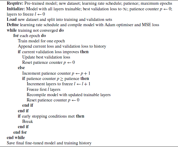
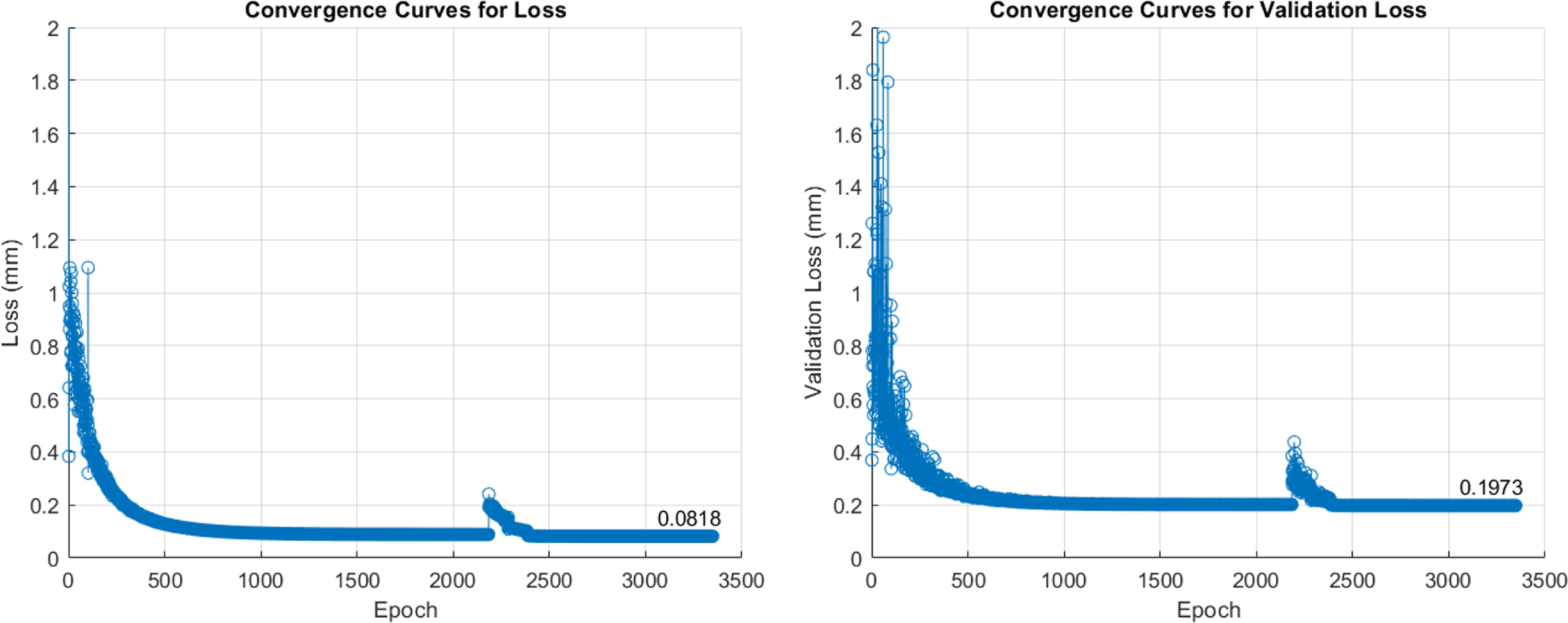
Figure 6. Fine-tuning results for Model 4 with 512 number of neurons.
Furthermore, in many application scenarios where multiple manipulators of different sizes (DH parameters) are required to complete a series of tasks, the proposed transfer learning algorithm can transfer the weights of an already trained model from one manipulator to another. This enables the rapid deployment and conversion of PMP models. Additionally, this kinematic transfer learning approach provides a convenient method for self-developed manipulators to utilise the algorithm to transfer known model weights to an unknown model. The only requirement is to have the manipulator move randomly within its workspace to collect data.
As illustrated above, the fine-tuned model was trained with data from the UR5e arm. Therefore, the proposed algorithm will transfer the model to the UR3 and UR10e arms separately. We used the same method to generate UR3 and UR10e data, each comprising half a million points. Subsequently, the training was conducted using the transfer learning algorithm and compared with the traditional direct training method. The comparison results are shown in Figure 7.
It is evident that convergence using transfer learning is significantly faster than with traditional methods. The initial loss value is lower in the transfer learning approach because the UR5 model is introduced first. In this experiment, from initial training to 1200th epoch, the validation loss for the UR3 converged from 33,472 to 0.1822 mm, and for the UR10e from 203,960 to 0.8725 mm using the traditional training method. In contrast, using transfer learning, the UR3 converged from 8.8140 to 0.0574 mm, and the UR10e converged from 2552.98 to 0.2203 mm. It is important to note that this transfer learning approach does not add additional algorithmic complexity to the training of the ANN, and its training efficiency remains comparable to that of the traditional method. However, the efficiency of the external training loop depends on the settings of the parameters, such as the number of epochs and the patience counter.

Figure 7. Comparison results between transfer learning and traditional training.
5.1. Discussion of results
In light of the above training results, it is clear that the activation function and network depth can impact the accuracy of approximating kinematic transformations using ANNs. This study found that the tanh function offers certain advantages in processing this type of data, and increasing the network depth can improve convergence speed to some extent. In practical applications, the working range of the robotic arm is usually fixed, so the training data collection can be limited to this range. Consequently, when the data does not encompass a large space, the model can be trained with fewer layers and reduced depth to save computational resources and decrease computational complexity when deploying the PMP. Additionally, although the final training accuracy of the ANN can achieve good accuracy, there is a possibility of over-fitting—whereby the robotic arm is only accurate within the space corresponding to the training data. If the workspace needs to be expanded, it is advisable to generate/collect new corresponding data and fine-tune the model again using transfer learning.
Regarding the transfer learning results, they indicate that when transferring from a large robotic arm to a smaller one (UR5e to UR3), the convergence speed is notably faster than when transferring from a smaller arm to a larger one (UR5e to UR10e). This is because the workspace of the larger arm encompasses that of the smaller arm. This observation reinforces the notion that the more complex the workspace, the more challenging it is to fit the data accurately.
6. Experiments and verification on the robotic arm
6.1. PMP-based movement implementation and analysis
As transfer learning can precisely approximate the kinematic transformation, the Jacobian matrix can be accurately evaluated based on the theory outlined in Section 2.2. In this section, the fine-tuned model based on Figure 6 is implemented in the PMP to evaluate the Jacobian matrix of the UR5e. Subsequently, the PMP model is verified on the physical UR5e robot. As shown in Figure 8, a common application scenario for a robotic arm involves acquiring the target position through sensors or cameras and then transmitting the target position to the controller, which drives the robot to reach the target. In this example, three separate targets were assigned, and their coordinate values (ground truth) and the actual positions reached by the robot are recorded in Table II. All coordinate points are referenced to the base of the arm, and the error is calculated as the Euclidean distance.
Table II. Experimental results of movements (unit: mm).
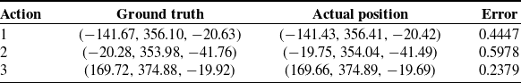

Figure 8. The experiment of UR5e: First, the initial position is set, then three target points are randomly assigned within the workspace, the target points are input to the PMP, and finally the PMP drive the robot to move from the initial position to the target sequentially.

Figure 9. Changes in the position of the end-effector and the angle of each joint during the movement from the initial point
 $(112.37, 334.54, 184.96)$
to the target.
$(112.37, 334.54, 184.96)$
to the target.
Additionally, throughout the PMP-solving process, the trajectories of the end-effector and the rotations of each joint angle of the robotic arm are plotted in Figure 9. As shown in the figure, the joint angles change smoothly, demonstrating the effectiveness of the PMP in computing feasible joint configurations for achieving the desired end-effector movement.
Figure 9 illustrates the joint angles and end-effector trajectories for three actions, each corresponding to a distinct end-effector position in 3D space. The left subplots show the evolution of joint angles over time, where most joints change continuously and smoothly to adapt to the required movement, while some undergo minor adjustments to stabilize the final pose. The right subplots depict the end-effector trajectories, which follow straight paths from the initial to the target positions. This linear movement reflects the constant and uniform stiffness matrix
 $ \mathbf {K}$
in Eq. (3) used during the experiment, ensuring a proportional force that drives the end-effector directly towards the target. The coefficient matrix is assumed constant throughout the analysis, meaning it does not depend on time or the system’s state. This assumption simplifies the model and facilitates the analysis of the resulting motion. In the simplest case, the stiffness matrix is proportional to the identity matrix, representing uniform stiffness in all directions. The stiffness matrix’s more complex, state- or time-dependent forms can also be considered.
$ \mathbf {K}$
in Eq. (3) used during the experiment, ensuring a proportional force that drives the end-effector directly towards the target. The coefficient matrix is assumed constant throughout the analysis, meaning it does not depend on time or the system’s state. This assumption simplifies the model and facilitates the analysis of the resulting motion. In the simplest case, the stiffness matrix is proportional to the identity matrix, representing uniform stiffness in all directions. The stiffness matrix’s more complex, state- or time-dependent forms can also be considered.
Across all three actions, the final joint (wrist 3) rotates from its initial configuration to achieve a consistent end-effector pose at the target. This final pose ensures that the gripper remains horizontal, aided by the constraints imposed by the admittance matrix
 $ \mathbf {A}$
in Eq. (5). The matrix effectively moderates the end-effector’s compliance, allowing the system to account for external disturbances and maintain the desired orientation.
$ \mathbf {A}$
in Eq. (5). The matrix effectively moderates the end-effector’s compliance, allowing the system to account for external disturbances and maintain the desired orientation.
The linear end-effector trajectories highlight the influence of constant stiffness, resulting in a direct force vector aiming at the target, with a magnitude proportional to the distance between the initial and target positions. Alternatively, by adjusting the stiffness matrix
 $ \mathbf {K}$
, it is possible to influence the trajectory of the end-effector, allowing it to follow a curved or more complex path. Such adjustments can be beneficial for avoiding obstacles around the environment.
$ \mathbf {K}$
, it is possible to influence the trajectory of the end-effector, allowing it to follow a curved or more complex path. Such adjustments can be beneficial for avoiding obstacles around the environment.
6.2. Comparisons results with MoveIt
Further, to compare with the approach built-in MoveIt, we present Table III, which records the results of both the PMP and MoveIt driving the UR5e to 10 additional randomly generated points under the same initial state. MoveIt uses a motion planning approach, which operates in the configuration space. It generates random samples and connects feasible configurations to construct a path, ensuring that the resulting joint angles yield minimal errors when achieving the desired end-effector position. While MoveIt performs better accuracy than PMP, it failed to generate a valid path in one instance, as shown in this table.
Table III. Comparison experiment results between MoveIt and PMP(unit: mm).

However, in many practical applications, the motion planning of a robotic arm also needs to consider some constraints, such as the expected pose of the robotic arm to reach the target, the magnitude of rotation of the joints, and so on. This enables obstacle avoidance or allows the end-effector to face the desired direction. Compared with MoveIt, the constraints could be straightforwardly imported using the admittance matrix without additional optimisation in the PMP approach. As shown in Figure 10, the images in the first row (a–c) are the results of MoveIt running without considering the constraints, compared to the initial state (yellow part), the end-effector orientations are all facing up while reaching the target. The other images (d–f) are the results of the PMP, when running these results, the fourth (wrist joint 1) and fifth joints (wrist joint 2) were constrained to 45 and 90 degrees by setting the admittance matrix, respectively. In other words, these results from PMP show that by introducing constraints, the arm can reach the target with an expected pose.

Figure 10. The UR5e motion planning in the simulation: the first row shows the planning results using MoveIt without constraints; the second row shows the PMP results with constraints.
Additionally, in this experiment, the same constraints were added to MoveIt, i.e., the two wrist joints were also set to 45 and 90 degrees, respectively, and a tolerance of
 $\pm 15$
degrees was allowed, but the algorithm reported that the planner could not find any valid states to reach the goal. While MoveIt excels at collision-free path planning, the PMP approach offers a simpler, more adaptive solution, particularly suited for applications prioritising smooth and compliant interaction adaptability.
$\pm 15$
degrees was allowed, but the algorithm reported that the planner could not find any valid states to reach the goal. While MoveIt excels at collision-free path planning, the PMP approach offers a simpler, more adaptive solution, particularly suited for applications prioritising smooth and compliant interaction adaptability.
6.3. Comparisons results with non-ANN based PMP
Furthermore, the proposed PMP method relies on an ANN implementation, as demonstrated by its ability to derive the Jacobian matrix and compute forward kinematics using trained weights. First, the Jacobian matrix serves as the critical link between the end-effector’s motion in extrinsic space and the joint velocities in intrinsic space. Its primary role in the PMP calculation loop is translating the positional displacement or force field into joint velocity or torque updates, driving the robot toward the target position. Second, the calculation loop also requires forward kinematics to determine the end-effector’s current position, which provides feedback for comparison with the intermediate target position. This intermediate target is generated as part of an integration process to ensure smooth progression towards the final goal (Eq. 7). Notably, the ANN-trained weights can substitute for both forward kinematics equations and Jacobian matrix derivation.
Admittedly, the forward kinematics and Jacobian matrix can also be solved analytically using the robot’s parameters. Therefore, in this section, the solution approach provided by the Robotics Toolbox will be used as an alternative to the ANN-based implementation for computing the Jacobian matrix and forward kinematics. This will enable a non-ANN-based PMP to be achieved and compared directly with the ANN-based PMP.
As the Robotics Toolbox has a built-in model of UR5, it will be used as the benchmark for comparison. The DH parameter of the UR5 in the Toolbox is shown in Table IV. Therefore, we transferred the trained UR5e model to the UR5 model for the ANN-based PMP, which used the same process described in Section 5. The other parts of the two algorithms remain the same, and the differences are the derivation of the Jacobian matrix and the forward kinematics solution.
The ANN model was retrained on data with the same joint angle ranges described in Section 4, establishing the working space for the trained ANN-based PMP. To evaluate performance, we randomly generated points within this working space and computed the results using both PMP algorithms. Each algorithm provided the final joint angles, which were then verified through forward kinematics using the DH parameters outlined in Table IV. The resulting positions and corresponding errors are recorded in Table V.
Table IV. DH parameters of the Robotics Toolbox’s UR5.

Table V. Comparison results between non-ANN-based PMP and ANN-based PMP in the defined working space(the initial position is
 $(91.23, 315.27, 118.60)$
, unit: mm)the initial state.
$(91.23, 315.27, 118.60)$
, unit: mm)the initial state.

Table VI. Comparison results between non-ANN-based PMP and ANN-based PMP in the defined working space(the initial position is
 $(\!-\!320.56, 226.71, 879.03)$
, unit: mm).
$(\!-\!320.56, 226.71, 879.03)$
, unit: mm).

Table VII. Comparison results between non-ANN-based PMP and ANN-based PMP outside the defined working space(the initial position is
 $(91.23, 315.27, 118.60)$
, unit: mm).
$(91.23, 315.27, 118.60)$
, unit: mm).

Notably, the PMP calculation loop requires comparing the current end-effector position with the target position to update the virtual force field. To demonstrate if the two algorithms are sensitive to the initial state, we changed the initial state of the UR5, i.e., the end-effector initial point was changed from
 $(91.23, 315.27, 118.60)$
to
$(91.23, 315.27, 118.60)$
to
 $(-320.56, 226.71, 879.03)$
, and reran the experiments of Table V. The new results are shown in Table VI.
$(-320.56, 226.71, 879.03)$
, and reran the experiments of Table V. The new results are shown in Table VI.
Compared with the two tables, the results showed that the ANN-based PMP is not sensitive to changes in the initial state. There are only minor differences in the computational results, and the overall performance of the ANN-based PMP is stable for different initial states. However, the non-ANN-based PMP illustrated significant sensitivity to the change in the initial state. This is probably because the non-ANN Jacobian computation suffers numerical instabilities or inaccuracies near singularities or at configurations requiring precise joint coordination. These discrepancies in the non-ANN Jacobian calculations can propagate through the PMP loop, resulting in cumulative errors. Especially, large differences between the initial and target positions may lead to further accumulating errors in the force field computation. Additionally, when the initial state changes, the intermediate target points of the integration trajectory also change, thus resulting in different solution accuracies.
In contrast, the ANN-based PMP is a data-driven model, and its performance depends on the distribution of training data within the working space. When the training data cover the full range of the working space, the model’s performance is robust. On the other hand, if training data does not fully cover the working space, the result should be unreliable. To demonstrate this, we reset the two PMP algorithms to the previous initial state
 $(91.23, 315.27, 118.60)$
under the same joint angles, and set the targets as outside points of the training working space, the results are shown in Table VII.
$(91.23, 315.27, 118.60)$
under the same joint angles, and set the targets as outside points of the training working space, the results are shown in Table VII.
Table VIII. Comparison results on the Sawyer Robot (the initial position is
 $(-207.5, 455.3, 619.25)$
, unit: mm).
$(-207.5, 455.3, 619.25)$
, unit: mm).
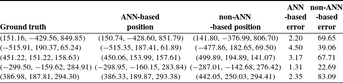
From the comparison results, it is clear that the ANN-based PMP significantly outperforms the non-ANN-based PMP within the working space. Conversely, outside the working space, the non-ANN-based PMP may be better, as it is independent of training data, relying on an idealised kinematic model. However, this reliance on a perfect model often fails to capture the physical robot’s behaviour accurately, leading to less precise joint angle outputs for certain positions. The instability or inaccuracy in the computation of the Jacobian matrix accumulates the error in the algorithm’s loop that struggles to ensure good accuracy.
Moreover, in most goal-directed actions, the arm must be coupled with an appropriate end-effector or tool, which is typically not incorporated into the arm’s forward kinematics. Tools might include a simple gripper, cutter, sprayer, or custom-designed and 3D-printed extensions. Therefore, generating data directly through robot experience to map motor commands and joint angles to their consequences (i.e., end-effector/tool positions) is necessary and advantageous. Such data can be generated kinesthetically or through imitation, eliminating the need for random exploration.
In the ANN-based PMP, the trained ANN effectively represents an internal model of the robot’s body, which is animated by the goal of synthesising the action. This enables a more robust and adaptive performance, particularly when the model is trained with comprehensive and representative data.
6.4. Implementation on the redundant manipulator
Finally, another ability of the PMP is that the computations are inherently well-posed, and its relaxation mechanism naturally resolves redundancy without requiring a cost function. This design ensures that indeterminacies related to excess degrees of freedom are handled implicitly through iterative updates of joint velocities guided by the force field and Jacobian matrix, allowing the system to converge to feasible solutions without explicit optimisation.
Therefore, we used the same method to build ANN-based PMP and non-ANN-based PMP models for a 7-degree-freedom robot, Sawyer Robot, and the comparison results are recorded in Table VIII. In this experiment, the trained ANN model of Sawyer Robot has an error of 1.67 mm on the validation set, the non-ANN model still uses the Robotics Toolbox to execute the Jacobian matrix and forward kinematic calculation. The experimental results were still conducted in the training workspace and the results once again validated that the ANN-based PMP has better accuracy in this scenario.
7. Conclusion
This paper implemented the PMP via deep neural networks and verified it on the UR series robots. First, the kinematic model based on the PMP is theoretically “well-posed,” eliminating the need to refer to and solve the inverse kinematics or additional optimisation and utilising impedance control and the equilibrium point hypothesis as alternatives to optimal control. Furthermore, the Jacobian matrix, as the core of the PMP, serves as the transformational “bridge” between the end-effector space and the joint space. Unlike traditional PMP models based on simple ANNs, this paper discusses the process of deriving the Jacobian matrix using deep neural networks, and the effects of the activation function and network depth are analysed. Subsequently, a transfer learning algorithm is proposed, which further optimises the pre-trained model and effectively facilitates the conversion of Jacobian matrix derivation models between different manipulators. Finally, the detailed experimental and comparison results demonstrated the feasibility, adaptability, and generalisability of the proposed method.
It is anticipated that future work will take advantage of new ANN architectures for the implementation of PMPs, such as long short-term memory [Reference Graves35] and transformer networks [Reference Vaswani, Shazeer, Parmar, Uszkoreit, Jones, Gomez, Kaiser and Polosukhin36], which may offer new insights into the derivation of Jacobian matrices based on ANNs. Further, the transfer learning method can be optimised to improve the re-training ability. Additionally, the current PMP is a position-driven model, which can be further developed into a force-driven model. This would enable the manipulator to reach the target and exert force on the target. Overall, PMP has considerable promise in both theory and application, and our future work will build upon this study.
Author contributions
FW conceived and designed the study. VM provided the theory and framework of the PMP. FW wrote the manuscript, and AT reviewed and approved this article.
Financial support
This research received no specific grant from any funding agency, commercial, or not-for-profit sectors.
Competing interests
The authors declare no competing interests exist.
Ethical approval
Not applicable.


